Zélus: A Synchronous Language with ODEs
Tutorial and Reference Manual
Release, version 1.2
École normale supérieure
45 rue d'Ulm
75230 Paris, France
Contents
-
Part I The Zélus Language
-
Chapter 1 Synchronous Programming
- 1.1 The Core Synchronous Language
- 1.2 Data types and Pattern Matching
- 1.3 Valued Signals
- 1.4 Hierarchical State Machines
- 1.4.1 Strong Preemption
- 1.4.2 Weak Preemption
- 1.4.3 Parameterized States
- 1.4.4 Modular Resets
- 1.4.5 Local State Definitions
- 1.4.6 States and Shared Memory
- 1.4.7 The Initial State
- 1.4.8 Resuming a State
- 1.4.9 Actions on Transitions
- 1.4.10 Signals and State Machines
- 1.4.11 Pattern Matching over Signals
- 1.5 Alternative Syntax for Control Structures
- 1.6 Real Time versus Logical Time
- Chapter 2 Hybrid Systems Programming
- Chapter 3 Compilation and Simulation
-
Chapter 1 Synchronous Programming
- Part II Reference manual
Foreword
Zélus is a synchronous language in the style of Lustre [12] and Lucid Synchrone [8] but extended to model hybrid systems that mix discrete-time and continuous-time signals. An example is a system that mix a (discrete-time) model of real-time control software that executes in closed loop with a model of its physical environment described by a Ordinary Differential Equations. More intricate interactions between discrete- and continuous-time behaviors can be expressed, like, for instance, continuous-time PID controllers or hybrid automata with several running modes, each of them being defined by an ODEs (the so-called hybrid automata). Zélus provides basic synchronous language constructs—difference and data-flow equations, hierarchical automata, and stream function definitions—in the style of Lustre [12] and Lucid Synchrone [8]. Continuous-time dymamics are expressed by ODEs with events defined as zero-crossings.
The expressiveness of the language is deliberately constrained to statically ensure determinism and the generation of loop-free sequential code that runs in bounded time and space. Moreover, code is generated identically for both embedded targets and simulation. For source programs with ODEs, the generated sequential code is paired with a numerical solver to approximate the continuous-time dynamics. Zélus’s main features are:
- It is a data-flow language in Single Static Assignment form: every name has only a single definition in the source code at any instant. A program is a collection of functions from signals to signals. A signal is a function from time to values. A set of signals is defined as the solution of a set of mutually recursive equations.
- The separation between discrete-time and continuous-time signals and
systems is imposed at the level of function definitions:
- A node is a function from discrete-time signals to discrete-time signals. A discrete-time signal is a sequence of values (a stream) as in other synchronous languages. A node is executed consecutively over the elements of a sequence of inputs to give a sequence of outputs. Nodes have no other notion of time than this succession of instants. In particular, there is no a priori ‘distance’ (time elapsed) between two instants. Outputs are produced atomically with triggering inputs, that is, instantaneously in the same discrete instant. They may depend on previous inputs; such nodes are termed stateful.
- A hybrid node is a function from continuous-time signals to continuous-time signals. A continuous-time signal is a signal defined on a sequence of time intervals on the real line. A hybrid node is executed on this set of instants. Only hybrid nodes may contain ODEs and detect zero-crossing events.
- All
discrete-time computations must be executed on a discrete clock.
This is statically enforced by the type system, following the convention:
A clock is termed discrete if it has been so declared or if it results from the sub-sampling a discrete clock or a zero-crossing. Otherwise, it is termed continuous.
It is possible to reset a continuous variable defined by an ODE on a discrete clock. A zero-crossing occurs when a continuous-time signal crosses zero from a negative value to a positive one during integration. Conceptually, a timer is a particular case of a zero-crossing event, even if the actual implementation is more specific.
- The basic types like integers, floating-point numbers, booleans, and characters are lifted from the host language OCaml. Abstract types, product types, record types, and enumerated types can either be defined directly or imported from the host language. Functions may have polymorphic types as in ML. Structured values are accessed via pattern matching.
- Data-flow equations may be composed arbitrarily with hierarchical automata as in Lucid Synchrone and SCADE 6. The compiler ensures determinacy and the absence of infinite loops. Hierarchical automata are internally rewritten into data-flow equations.
- The compiler is written in OCaml as a series of source-to-source and traceable transformations that ultimately yield statically scheduled sequential OCamlcode. The results of intermediate steps can be displayed. Continuous components are simulated using an off-the-shelf numerical solvers (SUNDIALS CVODE [13]) and, two built-in basic solvers (based on Matlab’s ode23 and ode45 solvers [18]).
Zélus is a research prototype that exhibits a new way of defining a hybrid systems modeling language based on the principles and techniques of synchronous languages. Its expressive power for modeling physics is limited to ODEs, unlike Modelica which is based on DAEs. Research papers on the design, semantics and implementation of Zélus are available at http://zelus.di.ens.fr.
Availability
The implementation is written in, and generates programs in OCaml, which must be installed.
| Zélus, version 1.2: | http://zelus.di.ens.fr |
| Objective Caml, version 4.02.1 | http://www.ocaml.org |
The language is experimental and evolves continuously. Please send comments or bug reports to Timothy.Bourke@inria.fr or Marc.Pouzet@ens.fr.
Copyright notice
This software includes the OCaml run-time system, which is copyrighted INRIA, 2015.
Thanks
This software is a research prototype that takes considerable time to develop. If you find it useful, please consider citing our work [6] and sending us comments.
Part I |
Chapter 1 Synchronous Programming
This chapter and the next one give a tutorial introduction to Zélus. This chapter focuses on the synchronous kernel of the language, which is reminiscent of Lustre and Lucid Synchrone. We shall sometimes compare Zélus with those two languages. The next chapter focuses on newer, hybrid aspects, like ODEs, zero-crossings, and their interaction with the synchronous features. The simulation engine is described in chapter 3.
Familiarity with general programming languages is assumed. Some familiarity with (strict or lazy) ML languages and with existing synchronous data-flow languages like Lustre is helpful but not mandatory. Some references are given at the end of this document.
In this tutorial, we suppose that programs are written in a file called
tutorial.zls.
1.1 The Core Synchronous Language
1.1.1 Point-wise Operations
Zélus is a first-order functional language. As in Lustre, every ground type or scalar value is imported from a host language (OCaml) and implicitly lifted to signals. A signal is a sequence or stream of values ordered in time: a value at an instant can only be produced after the values at all previous instants have been produced. This property models causality. In particular,
- int stands for the type of streams of integers,
- 1 stands for the constant stream of 1s,
- + stands for the pointwise addition operator over two input streams. It can be seen as an adder circuit just as && can be seen as an “and” gate.
Program executions can be represented as timelines showing the sequences of values taken by streams. The example below shows five streams, one per line. The first line shows a stream c, which has the value T (true) at the first instant, F (false) at the second one, and T at the third. The ‘⋯’ indicates that the stream has infinitely more values that are not shown. The next two lines define x and y. The fourth line defines a stream obtained by the pointwise addition of x and y. The expression in the fifth line takes the current value of either x or y according to the current value of c.
| c | true | false | true | ⋯ |
| x | x0 | x1 | x2 | ⋯ |
| y | y0 | y1 | y2 | ⋯ |
| x+y | x0 + y0 | x1 + y1 | x2 + y2 | ⋯ |
| if c then x else y | x0 | y1 | x2 | ⋯ |
1.1.2 Delays
The delay operator is denoted fby. The expression x fby y, which is read as “x followed by y” takes the first value of x at the first instant and the previous value of y at all instants thereafter. In other words, it delays y by one instant, and is initialized by x. This operator originated in the language Lucid [1].
| x | x0 | x1 | x2 | ⋯ |
| y | y0 | y1 | y2 | ⋯ |
| x fby y | x0 | y0 | y1 | ⋯ |
As it is often useful to separate a delay from its initialization, there is an operator pre x that delays its argument x and has an unspecified value (denoted here by nil) at the first instant. The complementary initialization operator x -> y takes the first value of x at the first instant, and the current value of y thereafter. The expression x -> (pre y) is equivalent to x fby y.
| x | x0 | x1 | x2 | ⋯ |
| y | y0 | y1 | y2 | ⋯ |
| pre x | nil | x0 | x1 | ⋯ |
| x -> y | x0 | y1 | y2 | ⋯ |
The compiler performs an initialization check to ensure that the behavior of a program never depends on the value nil. See section 1.1.9 for details.
Note:
A common error is to try to use the initialization operator to define the first two values of a stream. This does not work, since x -> y -> z = x -> z. One should instead write either x fby y fby z or x -> pre (y -> pre z). For example, the stream which starts with a value 1, followed by a 2, and then 3 forever is written 1 fby 2 fby 3 or 1 -> pre(2 -> pre(3)) or 1 -> pre(2 -> 3).
1.1.3 Global Declarations
A program is a sequence of declarations of global values. The keyword let defines non recursive global values which may be either constants or functions. For example:
let dt = 0.001
let g = 9.81
These declarations define two constant streams dt and g. Given the option -i, the compiler displays the types inferred for each declaration:
aneto.local: zeluc.byte -i tutorial.zls
Only constant values can be defined globally. The declaration
let first = true -> false
is rejected with the message:
aneto.local: zeluc.byte -i tutorial.zls
The right-hand side of a global let declaration may not contain delay operations. Definitions containing delays require the introduction of state. They may only be made within the node definition described in section 1.1.5.
1.1.4 Combinatorial Functions
Functions whose output at an instant depends only on inputs at the same instant are termed combinatorial. They are stateless and may thus be used in both discrete and continuous time. Any expression without delays, initialization operators, or automata is necessarily combinatorial.
As for any globally defined value, a combinatorial function is defined using the let keyword. Consider, for example, a function computing the instantaneous average of two inputs:
let average (x,y) = (x + y) / 2
The type signature inferred by the compiler, int * int -A-> int, indicates that it takes two integer streams and returns an integer stream. The arrow -A-> tagged with an A indicates that this function is combinatorial. The A stands for “any”—the function average can be used anywhere in the code. We will describe other possibilities soon.
Function definitions may contain local declarations, introduced using either where or let notations. For example, the average function can be written in two (equivalent) ways:
let average (x,y) = o where o = (x + y) / 2
and
let average (x,y) = let o = (x + y) / 2 in o
The full adder is a classic example of a combinatorial program. It takes three input bits, a, b, and a carry bit c, and returns outputs for the sum s and carry-out co.
let xor (a, b) = (a & not(b)) or (not a & b)

let full_add (a, b, c) = (s, co) where
       s = xor (xor (a, b), c)
   and co = (a & b) or (b & c) or (a & c)

Alternatively, a full adder can be described more efficiently as a composition of two half adders. A graphical depiction is given in figure 1.1. The corresponding program text is:
let half_add(a,b) = (s, co) where
       s = xor (a, b)
   and co = a & b
let full_add2(a, b, c) = (s, co) where
  rec (s1, c1) = half_add(a, b)
  and (s, c2) = half_add(c, s1)
  and co = c1 or c2
The rec keyword specifies that the block of equations following the where is defined by mutual recursion. Without it, the s1 in the equation for s and c2 would have to exist in the list of inputs or the global environment, and similarly for c1 and c2 in the equation for co.
Alternative notation:
For combinatorial function definitions, the keyword let can be replaced by fun.
fun half_add (a,b) = (s, co) where
  rec s = xor (a, b)
  and co = a & b
1.1.5 Stateful Functions
A function is stateful or sequential if its output at an instant n depends on the inputs at previous instants k (k ≤ n), that is, on the history of inputs. Such functions may produce a varying output signal even when their inputs are constant.
Stateful functions must be declared with the node keyword. For example, this function computes the sequence of integers starting at an initial value given by the parameter m:
let node from m = nat where
  rec nat = m -> pre nat + 1
The type signature int -D-> int indicates that from is a sequential function that maps one integer stream to another. The D indicates that this function is stateful, it stands for “discrete”. The function’s output may depend on the past values of its input.
Applying this function to the constant stream 0 yields the execution:
| m | 0 | 0 | 0 | 0 | 0 | 0 | ⋯ |
| 1 | 1 | 1 | 1 | 1 | 1 | 1 | ⋯ |
| pre nat | nil | 0 | 1 | 2 | 3 | 4 | ⋯ |
| pre nat + 1 | nil | 1 | 2 | 3 | 4 | 5 | ⋯ |
| m -> pre nat + 1 | 0 | 1 | 2 | 3 | 4 | 5 | ⋯ |
| from m | 0 | 1 | 2 | 3 | 4 | 5 | ⋯ |
The fact that a function is combinatorial is verified during compilation. Thus, omitting the node keyword,
let from n = nat where rec nat = n -> pre nat + 1
leads to an error message:
aneto.local: zeluc.byte -i tutorial.zls
While a node (arrow type -D->) cannot be called within a combinatorial function, it is possible to call a combinatorial function (arrow type -A->) within in a node. For example, the addition operator in the from function has the type signature int * int -A-> int.
We now present a few more examples of stateful functions.
The edge front detector is defined as a global function from boolean streams to boolean streams:
let node edge c = c & not (false fby c)
| c | false | false | true | true | false | true | ⋯ |
| false | false | false | false | false | false | false | ⋯ |
| false fby c | false | false | false | true | true | false | ⋯ |
| not (false fby c) | true | true | true | false | false | true | ⋯ |
| edge c | false | false | true | false | false | true | ⋯ |
A forward Euler integrator can be defined by:
let dt = 0.01
let node integr (x0, x') = x where
  rec x = x0 -> pre (x +. x' *. dt)
These declarations give a global function integr that returns a stream x defined recursively so that, for all n ∈ IN, x(n) = x0 + ∑i=0n−1 x′(i)· dt. The operators ‘+.’ and ‘*.’ are, respectively, addition and multiplication over floating-point numbers. Stateful functions are composed just like any other functions, as, for example, in:
let node double_integr (x0, x0', x'') = x where
  rec x = integr (x0, x')
  and x' = integr (x0', x'')
Alternative notation:
The keyword let can be omitted, for example,
let dt = 0.01
node integr (x0, x') = x where
  rec x = x0 -> pre (x +. x' *. dt)
1.1.6 Local and Mutually Recursive Definitions
Variables may be defined locally with let/in or let rec/in whether the defining expression is stateful or not. The following program computes the Euclidean distance between two points:
let distance ((x0,y0), (x1,y1)) =
  let d0 = x1 -. x0 in
  let d1 = y1 -. x1 in
  sqrt (d0 *. d0 +. d1 *. d1)
Since d0 and d1 denote infinite streams, the computations of x1 -. x0 and y1 -. x1 occur in parallel, at least conceptually. In Zélus, however, the consecutive nesting of let/ins introduces a sequential ordering on the computations at an instant. In this example, this means that the current value of d0 is always computed before the current value of d1. Being able to impose such an ordering is useful when functions with side-effects are imported from the host language. Write simply let rec d0 = ... and d1 = ... if no particular ordering is needed.
Streams may be defined through sets of mutually recursive equations. The function that computes the minimum and maximum of an input stream x can be written in at least three equivalent ways. As two mutually recursive equations after a where:
let node min_max x = (min, max) where
  rec min = x -> if x < pre min then x else pre min
  and max = x -> if x > pre max then x else pre max
as a stream of tuples defined by two local, mutually recursive equations:
let node min_max x =
  let rec min = x -> if x < pre min then x else pre min
      and max = x -> if x > pre max then x else pre max in
  (min, max)
or as a stream of tuples defined by a single recursive equation:
let node min_max x = (min, max) where
  rec (min, max) = (x, x) -> if x < pre min then (x, pre max)
                             else if x > pre max then (pre min, x)
                             else (pre min, pre max)
Discrete approximations to the sine and cosine functions can be defined by:
let node sin_cos theta = (sin, cos) where
  rec sin = integr(0.0, theta *. cos)
  and cos = integr(1.0, -. theta *. sin)
1.1.7 Shared Memory and Initialization
In addition to the delay operator pre, Zélus provides another construction for referring to the previous value of a stream: last o, where o is a variable defined by an equation. For example:
let node counter i = o where
  rec init o = i
  and o = last o + 1
The equation init o = i defines the initial value of the memory last o. This memory is initialized with the first value of i and thereafter contains the previous value of o. The above program is thus equivalent to the following one:1
let node counter i = o where
  rec last_o = i -> pre o
  and o = last_o + 1
The reason for introducing memories will become clear when control structures are introduced in section 1.2.2. Syntactically, last is not an operator: last o denotes a shared memory and the argument of last, here o, must be a variable name. Thus this program is rejected:
let node f () = o where
  rec o = 0 -> last (o + 1)
Rather than define the current value of a signal in terms of its previous one, the next value can also be defined in terms of the current one. The same counter program can be written:
let node counter i = o where
  rec init o = i
  and next o = o + 1
or equivalently:
let node counter i = o where
  rec next o = o + 1 init i
In both definitions, o is initialized with the first value of i and then the value of o at instant n+1 is the value of o + 1 at instant n (for all n ∈ IN).
Neither the form defining the current value from the previous one, nor the form defining the next value from the current one is intrinsically superior; it depends on the situation. Either form can be transformed into the other. We will see in chapter 2 that restrictions apply to both the next and last constructions when combining discrete- and continuous-time dynamics.
Remark: The compiler rewrites last, ->, fby, pre,
init and next into a minimal subset.
1.1.8 Causality Check
Instantaneous cycles between recursively defined values—causality loops—are forbidden so that the compiler can produce statically-scheduled sequential code. For example, the program:
let node from m = nat where
  rec nat = m -> nat + 1
is rejected with the message:
This program cannot be computed since nat depends instantaneously on itself. The compiler statically rejects function definitions that cannot be scheduled sequentially, that is, when the value of a stream at an instant n may be required in the calculation of that very value at the same instant, whether directly or through a sequence of intermediate calculations. In practice, we impose that all such stream interdependencies be broken by a delay (pre or fby). The purpose of causality analysis to to reject all other loops.
Note that delays can be hidden internally in the body of a function as is the case, for instance, in the languages Lustre and Signal. For example, consider the initial value problem:
|
We can approximate this value by using the explicit Euler integrator defined previously and defining a signal t by a recursive equation.
(* [t0] is the initial temperature; [g0] and [g1] two constants *)
let node heater(t0, g0, g1) = t where
  rec t = integr(t0, g0 -. g1 *. t)
This feedback loop is accepted because integr(t0, g0 -. g1 *. temp) does not depend instantaneously on its input.
It is also possible to force the compiler to consider a function as strict with the atomic keyword. For example, the following program is rejected by the causality analysis.
let atomic node f x = 0 -> pre (x + 1)
let node wrong () =
  let rec o = f o in o
Even though the output of f does not depend instantaneously on its input x, the keyword atomic adds instantaneous dependencies between the output and all inputs. For atomic functions, the compiler produces a single step function.2
1.1.9 Initialization Check
The compiler checks that every delay operator is initialized. For example,
let node from m = nat where
  rec nat = pre nat + 1
The analysis [10] is a one-bit analysis where expressions are considered to be either always defined or always defined except at the very first instant. In practice, it rejects expressions like pre (pre e), that is, uninitialized expressions cannot be passed as arguments to delays; they must first be initialized using the -> operator.
1.2 Data types and Pattern Matching
1.2.1 Type Definitions
Product types, record types, and enumerated types are defined in a syntax close to that of OCaml. Constructors with arguments are not supported in the current release. They can nevertheless be defined together with the functions that manipulate them in an OCaml module which is then imported into Zélus; see section 4.12.
Records are defined as in Ocaml and accessed with the dot notation. For example, the following defines a type circle, representing a circle as a record containing a center, given by its coordinates, and a radius.
type circle = { center: float ∗ float; radius: float }

let center c = c.center
let radius c = c.radius
1.2.2 Pattern Matching
Pattern matching over streams uses a match/with construction like that of OCaml.
For example, consider a colored wheel rotating on an axis for which we want to compute the direction of rotation. As shown in figure 1.2, the wheel has three sections with colors, ordered clockwise, blue (Blue), green (Green), and red (Red) . A sensor mounted on the frame detects the changing colors as the wheel turns.
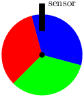
We must calculate whether the wheel is moving clockwise (Clockwise), that is, the sensor reports the sequence Red, Green, Blue, Red…, anticlockwise (Anticlockwise), whether it is not moving (Immobile), or whether the direction cannot be determined (Undetermined). We program the controller by first introducing two sum types:
type color = Blue | Red | Green
type dir = Clockwise | Anticlockwise | Undetermined | Immobile
The function direction then compares three successive values of the input stream i.
let node direction i = d where
  rec pi = i fby i
  and ppi = i fby pi
  and match ppi, pi, i with
      | (Red, Red, Red) | (Blue, Blue, Blue) | (Green, Green, Green) ->
             do d = Immobile done
      | (_, Blue, Red) | (_, Green, Blue) | (_, Red, Green) ->
             do d = Clockwise done
      | (_, Red, Blue) | (_, Green, Red) | (_, Blue, Green) ->
             do d = Anticlockwise done
      | _ -> do d = Undetermined done
  end
Each handler in a pattern-matching construct contains a set of equations defining shared variables; here the variable d. At each instant, the match/with statement in the example selects the first pattern (from the top) that matches the actual value of the triple ppi, pi, i and executes the corresponding branch. Only one branch is executed in any single reaction.
Combining such control structures with delay operators can give rise to subtle behaviors. Consider, for instance, the following program with two modes: in the Up mode, the variable o increases by 1 at each reaction and, in the mode Down, it decreases by 1.
type modes = Up | Down

let node two (m, i) = o where
  rec init o = i
  and match m with
      | Up -> do o = last o + 1 done
      | Down -> do o = last o - 1 done
      end
The equation init o = i defines a shared memory last o which is initialized with the first value of i. The variable o is called a shared variable because its definition is spread over several equations: when m equals Up, o equals last o + 1; when m equals Down, o equals last o - 1. Communication between the two modes occurs through the shared memory last o which contains the value that o had the last time that it was defined (that is, at the most recent previous instant of definition). An example execution diagram is given below.
| i | 0 | 0 | 0 | 0 | 0 | 0 | 0 | ⋯ |
| m | Up | Up | Up | Down | Up | Down | Down | ⋯ |
| last o + 1 | 1 | 2 | 3 | 3 | ⋯ | |||
| last o - 1 | 2 | 2 | 1 | ⋯ | ||||
| o | 1 | 2 | 3 | 2 | 3 | 2 | 1 | ⋯ |
| last o | 0 | 1 | 2 | 3 | 2 | 3 | 2 | ⋯ |
An equivalent way to express the same behaviour is:
let node two (m, i) = o where
  rec last_o = i -> pre o
  and match m with
      | Up -> do o = last_o + 1 done
      | Down -> do o = last_o - 1 done
      end
This version makes it clear how last o stands for the previously defined value of o.
The next section explains why using pre in this example would have given quite different results.
1.2.3 Pre versus Last
While last o may seem like just an alternative to pre o for referring to the previous value of a stream, there is a fundamental difference between the two based on their respective instants of observation.
- In Zélus, as in other block-diagram formalisms like Simulink and SCADE, pre e is a unit delay through a local memory—it denotes the value that its argument had the last time it was observed. If pre e is used in a block structure which is executed from time to time, for example, when some condition c is true, the argument e is only computed when c is true: pre e is the value of e the last time c was true.
- On the other hand, last o denotes the previous value of the variable o relative to the sequence of instants where the variable o (it must be a variable and not an expression) is defined. It is useful for communicating values between modes which is why it is called a shared memory.
We augment the previous example with extra equations to illustrate the difference between the two delay constructs. The two new streams c1 and c2 return respectively the number of instants in which each mode is active.
let node two (m, i) = (o, c1, c2) where
  rec init o = i
  and init c1 = 0
  and init c2 = 0
  and match m with
       | Up -> do o = last o + 1
               and c1 = 1 -> pre c1 + 1
               done
       | Down -> do o = last o - 1
                 and c2 = 1 -> pre c2 + 1
                 done
    end
The equation c1 = 1 -> pre c1 + 1 is only active in the Up mode, and the equation c2 = 1 -> pre c2 + 1 is only active in the Down mode. The execution diagram is given below.
| i | 0 | 0 | 0 | 0 | 0 | 0 | 0 | ⋯ |
| m | Up | Up | Up | Down | Up | Down | Down | ⋯ |
| last o + 1 | 1 | 2 | 3 | 3 | ⋯ | |||
| 1 -> pre c1 + 1 | 1 | 2 | 3 | 4 | ⋯ | |||
| last o - 1 | 2 | 2 | 1 | ⋯ | ||||
| 1 -> pre c2 + 1 | 1 | 2 | 3 | ⋯ | ||||
| o | 1 | 2 | 3 | 2 | 3 | 2 | 1 | ⋯ |
| last o | 0 | 1 | 2 | 3 | 2 | 3 | 2 | ⋯ |
| c1 | 1 | 2 | 3 | 3 | 4 | 4 | 4 | ⋯ |
| c2 | 0 | 0 | 0 | 1 | 1 | 2 | 3 | ⋯ |
Pattern matching composes complementary sub-streams. For instance, the match/with in the previous example has two branches, and each defines its own clock, one for the instants when m = Up and the other for the instants when m = Down.
1.2.4 Local Definitions
It is possible to define variables which are local to a branch. For example:
let node two (m, i) = o where
  match m with
  | Up -> let rec c = 0 -> pre c + 1 in
          do o = c done
  | Down -> do o = 0 done
  end
or equivalently:
let node two (m, i) = o where
  match m with
  | Up -> local c in
          do c = 0 -> pre c + 1
          and o = c done
  | Down -> do o = 0 done
  end
Here, c is declared local to the first handler of the match/with statement. The compiler verifies that a definition for c is given. Several variables can be declared local by writing local c1,..., cn in ....
1.2.5 Implicit Completion of Shared Variables
The branches of a pattern-matching construct need not contain definitions for all shared variables. Branches without a definition for a shared variable o are implicitly completed with an equation o = last o.
The compiler rejects programs where it is unable to ensure that last o has an initial value. The following program, for instance, is rejected.
let node two (m, i) = o where
  rec match m with
      | Up -> do o = last o + 1 done
      | Down -> do o = last o - 1 done
      end
1.3 Valued Signals
Zélus provides valued signals that are built and accessed, respectively, through the constructions emit and present. At every instant, a valued signal is a pair comprising (1) a boolean c indicating when the signal is present and (2) a value that is present when c is true.3
1.3.1 Signal Emission
Unlike shared variables, signal values are not necessarily defined at every instant, nor do they implicitly keep their previous value when not updated. Consider this program, for instance:
let node within (min, max, x) = o where
  rec c = (min <= x) & (x <= max)
  and present c -> do emit o = () done
It computes a condition c based on the input x. The signal o is present with value () every time c is true. There is no need to give an initial value for o. When c is false, o is simply absent. Removing the emit gives a program that the compiler rejects:
let node within (min, max, x) = o where
  rec c = (min <= x) & (x <= max)
  and present c -> do o = () done
The output o is not declared as a shared variable (with init) nor is it defined as a signal (with emit).
1.3.2 Signal Presence and Values
The presence of a signal expression e can be tested by the boolean expression ?e. The following program, for example, counts the number of instants where x is emitted.
let node count x = cpt where
  rec cpt = if ?x then 1 -> pre cpt + 1 else 0 -> pre cpt
There is also a more general mechanism to test signal presence that treats multiple signals simultaneously and allows access to their values. It resembles the pattern-matching construct of ML and it only allows signal values to be accessed at instants of emission.4
The program below has two input signals, x and y, and returns the sum of their values when both are emitted, the value of x when it alone is emitted, the value of y when it alone is emitted, and 0 otherwise.
let node sum (x, y) = o where
  present
  | x(v) & y(w) -> do o = v + w done
  | x(v) -> do o = v done
  | y(w) -> do o = w done
  else do o = 0 done
  end
A present statement comprises several signal patterns and handlers. The patterns are tested sequentially from top to bottom. The signal condition x(v) & y(w) matches when both x and y are present. The condition x(v) means “x is present and has some value v”. When x is present, the variable v is bound to its value in the corresponding handler.
In the signal pattern x(v) & y(w), x and y are expressions that evaluate to signal values and v and w are patterns. Writing x(42) & y(w) means “detect the presence of signal x with value 42 and the simultaneous presence of y”.
The output of the preceding function is a regular stream since the test is exhaustive thanks to the else clause. Omitting this default case results in an error.
let node sum (x, y) = o where
  present
  | x(v) & y(w) -> do o = v + w done
  | x(v1) -> do o = v1 done
  | y(v2) -> do o = v2 done
  end
This error is easily eliminated by giving a last value to o—for example, by adding the equation init o = 0 outside the present statement. The default case is then implicitly completed with o = last o. Another way is to state that o is a signal and thus only partially defined.
let node sum (x, y) = o where
  present
  | x(v) & y(w) -> do emit o = v + w done
  | x(v1) -> do emit o = v1 done
  | y(v2) -> do emit o = v2 done
  end
Signal patterns may also contain boolean expressions. The following program adds the values of the two signals x and y if they are emitted at the same time and if z >= 0.
let node sum (x, y, z) = o where
  present
    x(v) & y(w) & (z >= 0) -> do o = v + w done
  else do o = 0 done
  end
Remark: Signals make it possible to mimic the default construction of
the language Signal [4].
Signal’s default x y takes the value of x when x
is present and the value of y when x is absent and
y is present.
The signal pattern x(v) | y(v) tests the presence of “x or
y”.
let node signal_default (x, y) = o where
  present
    x(v) | y(v) -> do emit o = v done
  end
This is only a simulation of Signal’s behavior since all information about the instants where x and y are present—the so-called clock calculus of Signal [4]—is hidden at run-time and not exploited by the compiler. In particular, and unlike in the clock calculus of Signal, the Zélus compiler cannot determine that o is emitted only when x or y are present.
Unlike Lustre, Lucid Synchrone and Signal, Zélus does not currently have a clock calculus.
- 3
- For OCaml programmers: signals are like streams of an option type.
- 4
- Unlike in Esterel where signal values are maintained implicitly and can be accessed even in instants where they are not emitted. The approach of Zélus is slightly more cumbersome, but it is safer and avoids initialization issues and the allocation of a state variable.
1.4 Hierarchical State Machines
Zélus provides hierarchical state machines that can be composed in parallel with regular equations or other state machines as well as arbitrarily nested. State machines are essentially taken as is from Lucid Synchrone and SCADE 6. They are compiled to data-flow equations [9].
In this tutorial, we first consider basic state machines where transition guards are limited to boolean expressions. We then consider two important extensions. The first is the ability to define state machines with parameterized states (section 1.4.3) and actions on transitions (section 1.4.9). The second is a more general form of transitions with signal matching and boolean expressions (section 1.4.11).
An automaton is a collection of states and transitions. Two kinds of transitions are provided: weak and strong. For each, it is possible to enter the next state by reset or by history. An important feature of state machines in Zélus is that only one set of equations is executed during any single reaction.
1.4.1 Strong Preemption
The following program contains a two state automaton with strong preemption, it returns false until x becomes true and then it returns true indefinitely.
let node strong x = o where
  automaton
  | S1 -> do o = false unless x then S2
  | S2 -> do o = true done
  end
Each of the two states defines a value for the shared variable o. The keyword unless indicates a strong transition: the automaton stays in the state S1 as long as x is false, and o is defined by the equation o = false, but the instant that x becomes true, S2 becomes active immediately, and o is defined by the equation o = true. Thus, the following timeline holds:
| x | false | false | true | false | false | true | ⋯ |
| strong x | false | false | true | true | true | true | ⋯ |
The guards of strong transitions are tested before determining which state is active at an instant and executing its body.
1.4.2 Weak Preemption
The following program contains a two state automaton with weak preemption, it returns false at the instant that x becomes true and then it returns true indefinitely; it is like a Moore automaton.
let node expect x = o where
  automaton
  | S1 -> do o = false until x then S2
  | S2 -> do o = true done
  end
This timeline of this program is shown below.
| x | false | false | true | false | false | true | ⋯ |
| expect x | false | false | false | true | true | true | ⋯ |
The guards of weak transitions are tested after executing the body of the current active state to determine the active state at the next instant.
We now consider a two state automaton that switches between two states whenever the input toggle is true.
let node weak_switch toggle = o where
  automaton
  | False -> do o = false until toggle then True
  | True  -> do o = true until toggle then False
  end
For an example input stream, the timeline is:
| toggle | false | true | false | false | true | true | false | ⋯ |
| o | false | false | true | true | true | false | true | ⋯ |
The form with strong transitions follows.
let node strong_switch toggle = o where
  automaton
  | False -> do o = false unless toggle then True
  | True  -> do o = true unless toggle then False
  end
Its behavior relative to the same input sequence differs.
| toggle | false | true | false | false | true | true | false | ⋯ |
| o | false | true | true | true | false | true | true | ⋯ |
In fact, for any boolean stream toggle the following property holds:
let node correct toggle =
weak_switch toggle = strong_switch (false -> pre toggle)

The graphical representations of these two automata are shown in figure 1.3. The circles on the transition arrows distinguish weak transitions from strong ones: they graphically separate the actions of one instant from another. Since a weak transition is executed in the same instants as its source state, the circle is placed to separate it from its destination state. Since a strong transition is executed in the same instants as its destination state, the circle is placed to separate it from its source state.
Remark: The current version of Zélus does not permit arbitrary
combinations of weak and strong transitions within an automaton as in
Lucid Synchrone and SCADE 6.
After much experience with automata, we think that such arbitrary mixes give
programs that are difficult to understand.
Future versions of Zélus may, however, allow a constrained mix of weak
and strong transitions.
1.4.3 Parameterized States
In the examples considered so far, each automaton had a finite set of states and transitions. It is also possible to define more general state machines with parameterized states, that is, states containing local values that are initialized on entry. Parameterized states are a natural way to pass information between states and to reduce the number of explicitly programmed states. Parameterized state machines lead to a style of programming that resembles the definition of mutually tail-recursive functions in ML. Yet they are not compiled into mutually recursive functions but into a single step function with a switch-like construct over the active state.
In the following function, the automaton waits in its initial state for the signal e. When e is present, its value is bound to v and the automaton transitions to the state Sustain(v), that is, to the state Sustain with parameter x set to v.
(* wait for e and then sustain its value indefinitely *)
let node await e = o where
  automaton
  | Await -> do unless e(v) then Sustain(v)
  | Sustain(x) -> do emit o = x done
  end
The formal parameter x of the Sustain state can be used without restriction in the body of the state, and the variable v could just as well have been an expression.
As another example, the program below uses parameterized states to count the occurrences of x. It simulates an infinite state machine with states Zero, Plus(1), Plus(2), etcetera.
let node count x = o where rec o = 0 -> pre o + 1

let node count_in_an_automaton x = o where
  automaton
  | Zero    -> do o = 0 until x then Plus(1)
  | Plus(v) -> do o = v until x then Plus(v+1)
  end
1.4.4 Modular Resets
Gérard Berry’s ABRO example highlights the expressive power of parallel composition and preemption in Esterel. The specification is [5, §3.1]:
Emit an output O as soon as two inputs A and B have occurred. Reset this behavior each time the input R occurs.
We will implement this example in Zélus—replacing uppercase letters by lowercase ones5—but generalize it slightly by considering valued events.
As a first step, consider a function that implements the first part of the specification: it waits for occurrences of both a and b using the await node from section 1.4.3 and then emits the sum of their values.
let node abo (a, b) = o where
  present (await a)(v1) & (await b)(v2) -> do emit o = v1 + v2 done
This first version is readily extended to the full specification by putting it inside an automaton state with a self-looping (weak) transition that resets it when r is true.
let node abro (a, b, r) = o where
  automaton
  | S1 ->
       do
         present (await a)(v1) & (await b)(v2) -> do emit o = v1 + v2 done
       unless r then S1
  end
A graphical version is shown in figure 1.4. The transition on r resets the computation within the state: all streams in abo a b, including those inside both await nodes, restart with their initial values.
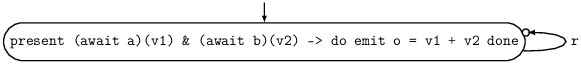
Zélus also provides a specific reset/every primitive as a shortcut for such a one-state automaton. It combines a set of parallel equations (separated by ands). We could thus write:
let node strong_abro (a, b, r) = o where
  reset
    present (await a)(v1) & (await b)(v2) -> do emit o = v1 + v2 done
  every r
Except that reset/every is strongly preemptive; the body is reset before being executed at the instant the condition is true. There is no “weak reset” since one need only add a unit delay for the same effect. The following program implements the ABRO specification.
let node abro (a, b, r) = o where
reset
  o = abo (a, b)
every true fby r
1.4.5 Local State Definitions
Names may be declared local to a state. Such names can only be used inside the body of the state and in the guards of outgoing weak transitions.
The following program sums the integer sequence v and emits false until the sum has reached some value max. Then, it emits true for n instants.
let node consume (max, n, v) = status where
  automaton
  | S1 ->
      let rec c = v -> pre c + v in
      do status = false
      until (c = max) then S2
  | S2 ->
      let rec c = 1 -> pre c + v in
      do status = true
      until (c = n) then S1
  end
State S1 defines a local variable c that is used to compute the weak condition c = max without introducing any causality problems. Indeed, weak transitions only take effect in a subsequent reaction: they define the next state, not the current one. Moreover, there is no restriction on the kind of expressions appearing in conditions and they may, in particular, have some internal state. For example, the previous program can be rewritten as:
let node sum v = cpt where
  rec cpt = v -> pre cpt + v

let node consume (max, n, v) = status where
  automaton
  | S1 ->
       do status = false
       until (sum v = max) then S2
  | S2 ->
       do status = true
       until (sum 1 = n) then S1
  end
The body of a state comprises (possibly empty) sequences of local declarations (with local/in), local definitions (with let/in), and definitions of shared variables (with do/until). As noted previously, weak conditions may depend on local names and shared names.
In weak preemptions, as in the example above, transition conditions are evaluated after the equations in the body have been evaluated. The untils in this example may not be replaced with unlesss because in strong preemptions the transition conditions are evaluated before the equations in the body and may not depend on them. Thus, writing
let node consume (max, n, v) = status where
  automaton
  | S1 ->
      let rec c = v -> pre c + v in
      do status = false
      unless (c = max) then S2
  | S2 ->
      let rec c = 1 -> pre c + 1 in
      do status = true
      unless (c = n) then S1
  end
causes the compiler to emit the message:
The variable c is not visible in the handler of the unless. The same problem occurs if c is declared as a local variable, as in the following program.
let node consume (max, n, v) = status where
  automaton
  | S1 ->
      local c in
      do c = v -> pre c + v and status = false
      unless (c = max) then S2
  | S2 ->
      local c in
      do c = v -> pre c + v and status = true
      unless (c = n) then S1
  end
1.4.6 States and Shared Memory
In the previous examples, there is no communication between the values computed in each state. We now consider the following simple system, due to Maraninchi and Rémond [16], of two running modes.
let node two_states (i, min, max) = o where
  rec automaton
      | Up -> do o = last o + 1
              until (o = max) then Down
      | Down -> do o = last o - 1
                until (o = min) then Up
      end
  and init o = i
In the Up mode, the system continually increments some value by 1 and in the Down mode, it decrements the same value by the same amount. The transitions between these two modes are described by a two-state automaton whose behavior depends on the value computed in each mode. The system’s execution diagram is
| i | 0 | 0 | 0 | 0 | 0 | 0 | 0 | 0 | 0 | 0 | 0 | 0 | … |
| min | 0 | 0 | 0 | 0 | 0 | 0 | 0 | 0 | 0 | -1 | 0 | 0 | … |
| max | 4 | 4 | 4 | 4 | 4 | 4 | 4 | 4 | 4 | 4 | 4 | 4 | … |
| o | 1 | 2 | 3 | 4 | 3 | 2 | 1 | 0 | -1 | 0 | 1 | 2 | … |
| last o | 0 | 1 | 2 | 3 | 4 | 3 | 2 | 1 | 0 | -1 | 0 | 1 | … |
| last o + 1 | 1 | 2 | 3 | 4 | 0 | 1 | 2 | … | |||||
| last o - 1 | 3 | 2 | 1 | 0 | -1 | … |
As for match/with and present, an implicit completion mechanism applies so that variables like o need not be explicitly defined in all automaton states. When an equation is not given, the shared variable keeps its previous values. In other words, an equation o = last o is assumed.
1.4.7 The Initial State
The initial automaton state can be used to define the values of variables that are shared across the other states. Such variables are considered to have a last value that can be accessed through the last operator. And, thanks to o = last o completion, explicit definitions can be omitted in other states.
let node two_states (i, min, max) = o where
  rec automaton
      | Init ->
           do o = i until (i > 0) then Up
      | Up ->
          do o = last o + 1
          until (o = max) then Down
      | Down ->
          do o = last o - 1
          until (o = min) then Up
      end
| i | 0 | 0 | 0 | 1 | 1 | 1 | 1 | 1 | 1 | 1 | 1 | 1 | 1 | 1 | 1 | … |
| min | 0 | 0 | 0 | 0 | 0 | 0 | 0 | 0 | 0 | 0 | 0 | 0 | -1 | 0 | 0 | … |
| max | 0 | 0 | 0 | 4 | 4 | 4 | 4 | 4 | 4 | 4 | 4 | 4 | 4 | 4 | 4 | … |
| o | 0 | 0 | 0 | 1 | 2 | 3 | 4 | 3 | 2 | 1 | 0 | -1 | 0 | 1 | 2 | … |
| last o | 0 | 0 | 0 | 0 | 1 | 2 | 3 | 4 | 3 | 2 | 1 | 0 | -1 | 0 | 1 | … |
| last o + 1 | 0 | 0 | 0 | 1 | 2 | 3 | 4 | 0 | 1 | 2 | … | |||||
| last o - 1 | 0 | 0 | 0 | 3 | 2 | 1 | 0 | -1 | … |
As the initial state Init is only weakly preempted, o is necessarily initialized with the current value of i. Thus, last o is well defined in the remaining states. Replacing weak preemption by strong preemption results in an error.
let node two_states (i, min, max) = o where
  rec automaton
      | Init ->
          do o = i unless (i > 0) then Up
      | Up ->
          do o = last o + 1
          unless (o = max) then Down
      | Down ->
          do o = last o - 1
          unless (o = min) then Up
      end
As explained in section 1.4.5, the guards of strong transitions may not depend on variables computed in the current state. They may depend, however, on a shared memory last o, as in:
let node two_states (i, min, max) = o where
rec init o = i
and automaton
      | Init ->
          do o = i unless (i > 0) then Up
      | Up ->
          do o = last o + 1
          unless (last o = max) then Down
      | Down ->
          do o = last o - 1
          unless (last o = min) then Up
      end
giving the same execution diagram as before:
| i | 0 | 0 | 0 | 1 | 1 | 1 | 1 | 1 | 1 | 1 | 1 | 1 | 1 | 1 | 1 | … |
| min | 0 | 0 | 0 | 0 | 0 | 0 | 0 | 0 | 0 | 0 | 0 | 0 | -1 | 0 | 0 | … |
| max | 0 | 0 | 0 | 4 | 4 | 4 | 4 | 4 | 4 | 4 | 4 | 4 | 4 | 4 | 4 | … |
| o | 0 | 0 | 0 | 1 | 2 | 3 | 4 | 3 | 2 | 1 | 0 | -1 | 0 | 1 | 2 | … |
| last o | 0 | 0 | 0 | 0 | 1 | 2 | 3 | 4 | 3 | 2 | 1 | 0 | -1 | 0 | 1 | … |
| last o + 1 | 0 | 0 | 0 | 1 | 2 | 3 | 4 | 0 | 1 | 2 | … | |||||
| last o - 1 | 0 | 0 | 0 | 3 | 2 | 1 | 0 | -1 | … |
An initial state may be parameterized if an explicit initialization clause is added to the automaton. For example, the following two state automaton starts in state Run(incr) with incr initialized to the first value of i0.
let node two_states(i0, idle, r) = o where
  rec automaton
      | Run(incr) ->
          do o = 0 fby o + incr until idle() then Idle
      | Idle ->
          do until r(incr) then Run(incr)
      init Run(i0)
1.4.8 Resuming a State
By default, the computations within an automaton state are reset when it is entered. So, for instance, the counters in the states of the example below are reset on every transition.
let node time_restarting c = (x, y) where
  rec automaton
      | Init ->
          do x = 0 and y = 0 then S1
      | S1 ->
          do x = 0 -> pre x + 1 until c then S2
      | S2 ->
          do y = 0 -> pre y + 1 until c then S1
      end
Giving the execution trace (where we write F for false and T for true):
| c | F | F | F | F | T | F | T | F | F | F | F | T | T | F | F | F |
| x | 0 | 0 | 1 | 2 | 3 | 3 | 3 | 0 | 1 | 2 | 3 | 4 | 4 | 0 | 1 | 2 |
| y | 0 | 0 | 0 | 0 | 0 | 0 | 1 | 1 | 1 | 1 | 1 | 1 | 0 | 0 | 0 | 0 |
Note that the transition from the initial state, do x = 0 and y = 0 then S1, is shorthand for do x = 0 and y = 0 until true then S1.
It is also possible to enter a state without resetting its internal memory (as in the entry-by-history of StateCharts) using the continue transitions. The modified example,
let node time_sharing c = (x, y) where
  rec automaton
      | Init ->
          do x = 0 and y = 0 continue S1
      | S1 ->
          do x = 0 -> pre x + 1 until c continue S2
      | S2 ->
          do y = 0 -> pre y + 1 until c continue S1
      end
has the execution trace:
| c | F | F | F | F | T | F | T | F | F | F | F | T | T | F | F | F |
| x | 0 | 0 | 1 | 2 | 3 | 3 | 3 | 4 | 5 | 6 | 7 | 8 | 8 | 9 | 10 | 11 |
| y | 0 | 0 | 0 | 0 | 0 | 0 | 1 | 1 | 1 | 1 | 1 | 1 | 2 | 2 | 2 | 2 |
This is a way of writing activation conditions. It is convenient, for instance, for programming a scheduler which alternates between different computations, each of them having its own state.
1.4.9 Actions on Transitions
It is possible to perform an action on a transition. As an example, consider programming a simple mouse controller with the following specification.
Return the event double whenever two clicks are received in less than four tops. Emit simple if only one click is received within the interval.
Here is one possible implementation:
let node counting e = cpt where
  rec cpt = if e then 1 -> pre cpt + 1 else 0 -> pre cpt
let node controller (click, top) = (simple, double) where rec
  automaton
  | Await ->
     do simple = false and double = false until click then One
  | One ->
     do until click then do simple = false and double = true in Await
     else (counting top = 4) then
        do simple = true and double = false in Await
  end
This program waits for the first occurrence of click, then it enters the One state and starts to count the number of tops. This state is exited when a second click occurs or when the condition counting top = 4 becomes true.
Note that the One state has two outgoing weak transitions (the second prefixed by else. As for the present construct, transition guards are evaluated in order from top to bottom. The first to be satisfied is triggered.
| click | F | T | F | T | F | T | F | F | F | F | F | F | F | F |
| top | T | F | T | F | T | T | F | T | T | T | F | T | T | F |
| simple | F | F | F | F | F | F | F | F | F | F | F | T | F | F |
| double | F | F | F | T | F | F | F | F | F | F | F | F | F | F |
Any set of equations can be placed between the do/in of a transition, exactly as between a do/until or do/unless.
1.4.10 Signals and State Machines
In the automata considered until now, the conditions on transitions have been boolean expressions. The language also provides a more general mechanism for testing signals and accessing their values on transitions.
Using signals, we can reprogram the mouse controller of the previous section as follows.
type event = Simple | Double

let node controller (click, top) = o where
  automaton
  | Await ->
     do until click then One
  | One ->
     do until click then do emit o = Double in Await
        else (counting top = 4) then do emit o = Simple in Await
  end
This time no variables are defined in state Await. Writing emit o = x means that o is a signal and not a regular stream, there is thus no need to define it in every state of the automaton nor to declare a last value. The signal o is only emitted in state Emit. Otherwise, it is absent.
| click | F | T | F | T | F | T | F | F | F | F | F | F | F | F |
| top | T | F | T | F | T | T | F | T | T | T | F | T | T | F |
| o | Double | Simple |
Combining signals with a sum type, as is done here, has some advantages over the use of boolean variables in the original program. By construction, only three values are possible for the output: o can only be Simple, Double or absent. In the previous version, a fourth case corresponding to the boolean value simple & double is possible, even though it is meaningless.
1.4.11 Pattern Matching over Signals
The signal patterns introduced in section 1.3.2 for the present construct may also be used in transition conditions to combine signals and access their values.
Consider, for example, the system below that has two input signals inc and dec, and that outputs a stream of integers o.
let node switch (inc, dec) = o where
  rec automaton
      | Init ->
          do o = 0
          until inc(u) then Up(u)
           else dec(u) then Down(u)
      | Up(u) ->
          do o = last o + u
          until dec(v) then Down(v)
      | Down(v) ->
          do o = last o - v
          until inc(u) then Up(u)
      end
The condition until inc(u) means: await the presence of the signal low with some value u, then transition to the parameterized state Up(u).
A basic preemption condition has the form e(p) where e is an expression of type t sig and p is a pattern of type t. The condition binds the variables in the pattern p from the value of the signal at the instant when e is present. In the above example, for instance, the variable u is introduced and bound over the rest of the transition. A test for signal presence can be combined with a boolean condition. For example,
let node switch (inc, dec) = o where
  rec automaton
  | Init ->
      do o = 0
      until inc(u) then Up(u)
       else dec(u) then Down(u)
  | Up(u) ->
      let rec timeout = 0 -> pre timeout + 1 in
      do o = last o + u
      until dec(v) & (timeout > 42) then Down(v)
  | Down(v) ->
      let rec timeout = 0 -> pre timeout + 1 in
      do o = last o - v
      until inc(u) & (timeout > 42) then Up(u)
  end
This system has the same behavior except that the presence of dec in the Up state is only taken into account when the timeout stream has passed the value 42.
- 5
- As in OCaml, identifiers starting with an uppercase letter are considered to be data type constructors and cannot be used as variable names.
1.5 Alternative Syntax for Control Structures
Each of the three control structures (match/with, automaton, and present) combines equations. Each branch comprises a set of equations defining shared values. In this form, it is not necessary to explicitly define all shared variables in every branch since they implicitly keep their previous value or, for signals, become absent.
This syntactical convention mirrors the graphical representation of programs in synchronous dataflow tools (like SCADE). In such tools, control structures naturally combine (large) sets of equations and the implicit completion of absent definitions is essential.
The language also provides a derived form that allows control structures to be used in expressions. For example,
let node two x =
  match x with | true -> 1 | false -> 2
can be written as a shorthand for
let node two x =
  let match x with
     |  true -> do o = 1 done
     | false -> do o = 2 done
     end in
  o
This notation is more conventional for OCaml programmers. A similar shorthand exists for the present and automaton constructs. One can write, for instance,
let node toggle x = y where
  rec y =
    automaton
    | S0 -> do 0 until x then S1
    | S1 -> do 1 until x then S0
1.6 Real Time versus Logical Time
We close the chapter on synchronous programming with an example real-time controller that tracks the passage of time using counters that then influence the running mode. This example highlights the difference between the idea of logical time considered thus far and that of real-time.
Consider a light that blinks according to the specification:
Repeat the following behavior indefinitely: Turn a light on for n seconds and then off for m seconds. Allow it to be restarted at any instant.
One way to start implementing this specification is to define a boolean signal called second that is true at every occurrence of a second, whatever that may mean, and false otherwise. We then define a node called after_n(n, t) that returns true when n true values are counted on t. This is then instantiated twice in a node called blink_reset containing an automaton with two modes wrapped by a reset construct.
let node after_n(n, t) = (cpt >= n) where
  rec tick = if t then 1 else 0
  and ok = cpt >= n
  and cpt = tick -> if pre ok then n else pre cpt + tick

let node blink_reset (restart, n, m, second) = x where
 reset
   automaton
   | On  -> do x = true  until (after_n(n, second)) then Off
   | Off -> do x = false until (after_n(m, second)) then On
 every restart
The type signatures inferred by the compiler are:
Does after_n(n, second) really give a delay of n real-time seconds? No, for two reasons (see also [7]):
- second is a Boolean stream. No hypothesis is made or ensured by the compiler about the actual real-time duration between two occurrences of true in the stream. It is up to the implementation to ensure that second correctly approximates a real second.
- The counting of instants in the expression after_n(n, t) is only performed when the expression is active, that is, it returns true when n occurrences of the value true have been observed. This can be less than the number of occurrences of the value true of n. E.g., instantiating blink_reset within a branch of an automaton or match that is activated from time to time.
In this chapter, time is logical meaning that we count number of occurrences. We shall see in the next chapter how to connect it with physical time.
Chapter 2 Hybrid Systems Programming
In this chapter we introduce the main novelty of Zélus with respect to standard synchronous languages: all of the previously introduced constructs, that is, stream equations and hierarchical automata, can be combined with Ordinary Differential Equations (ODEs). As before, we only present basic examples in this document. More advanced examples can be found on the examples web page.
2.1 Initial Value Problems
Consider the classic Initial Value Problem that models the temperature of a boiler. The evolution of the temperature t is defined by an ODE and an initial condition:
|
where g0 and g1 are constant parameters and t0 is the initial temperature. Instead of choosing an explicit integration scheme as in section 1.1.8, we can now just write the ODE directly:
let hybrid heater(t0, g0, g1) = t where
  rec der t = g0 -. g1 *. t init t0
The der keyword defines t by a (continuous) derivative and an initial value. Notice that the hybrid keyword is used here rather than node. It signifies the definition of a function between continuous-time signals. This is reflected in the type signature inferred by the compiler with its -C-> arrow. The C stands for “continuous” Hybrid functions need special treatment for simulation with a numeric. Discrete nodes, on the other hand, evolve in logical time, that is, as a sequence of instants, and may not contain any nested continuous-time computations.
As a second example of the new features, consider the following continuous definition of the sine and cosine signals whose stream approximation was given in section 1.1.6:
let hybrid sin_cos theta = (sin, cos) where
  rec der sin = theta *. cos init 0.0
  and der cos = -. theta *. sin init 1.0
Are these definitions really all that different from those in the previous chapter? Yes!
The dynamics of the boiler temperature and those of the sine and cosine
signals are now defined by ODEs, and a numeric solver is used to approximate
their continuous-time trajectories.
The choice of the solver is independent of the model and made outside the
language.
Programs are defined at a higher level of abstraction, leaving the choice of
an integration scheme to the numerical solver.
In particular, signals are not necessarily integrated using a fixed-step
explicit scheme like that coded manually in section 1.1.8.
It is possible to program models that mix discrete-time computations with
ODEs and to simulate them together using an external solver.
Remark: The compiler generates sequential code that allows ODEs to be
approximated by a numerical solver.
The current version of Zélus provides an interface to the
Sundials
CVODE [13]
solver and two classical variable step solvers (ode23 and
ode45 [11]).
A Proportional Integral (PI) controller is a classic example of a
continuous-time function.
Below we present two implementations: a continuous version to be
approximated by an external numeric solver, and a discrete version using
forward Euler integration.
(* a continuous-time integrator *)
let hybrid integr(x0, x') = x where
  rec der x = x' init x0

(* a continuous-time PI controller *)
let hybrid pi(kp, ki, error) = command where
  rec command = kp *. error +. ki *. integr(0.0, error)

let ts = 0.05

(* a explicit Euler integration *)
let node disc_integr(y0, x') = y where
  rec y = y0 -> last y +. ts *. x'

(* a discrete-time PI controller *)
let node disc_pi(kp, ki, error) = cmd where
  rec cmd = kp *. error +. ki *. disc_integr(0.0, error)
2.2 Mixing Discrete and Continuous Signals
Care must be taken when mixing signals and systems defined in discrete logical time with those defined in continuous time, both to ensure that programs make sense and that they can be simulated effectively. Consider, for instance, the following simple program.
let hybrid wrong1() = o where
  rec der x = 1.0 init 0.0
  and o = 0.0 -> pre o +. x
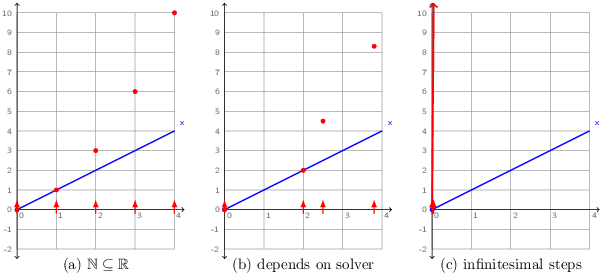
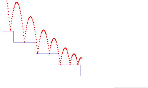
The signal x is continuous and o is discrete (due to the -> and pre operators). What can it mean to put them in parallel in this way? The meaning of x along is clear: ∀ t ∈ ℝ+, x(t) = t. It is shown in the three diagrams of figure 2.1 as a blue line that increases from zero with a constant slope. Each of the diagrams shows a different interpretation for o:
- Since the discrete reactions can be numbered by the natural numbers and these numbers are a subset of the reals, we could decide to simply embed the discrete reactions at times 0.0, 1.0, 2.0, etcetera. The value of o is then perfectly well defined (the red dots in the figure), but the mapping of reactions to continuous time is completely arbitrary.
- Since a numeric solver must inevitably approximate continuous signals over a sequence of discrete steps, we could decide to execute discrete equations at the sampling instants chosen by the solver. This mapping of reactions is less arbitrary since it corresponds to the underlying discrete solver process, but the meaning of a program now depends on low-level details of the numerical simulation. Changing the solver or its parameters, or adding another unrelated equation in parallel will likely change the value of o.
- A third possibility is to consider that the process corresponding to o is iterated continually, that is, as time advances infinitesimally. Although the value of o rapidly diverges toward infinity, it is well defined. The real problem is that such programs cannot be effectively simulated using numeric techniques.
We do not consider any of these three alternatives as acceptable. Instead, the compiler rejects wrong1 as invalid:
Similarly, a second program,
let hybrid wrong2() = o where
  rec der x = o init 0.0
  and o = 0.0 -> pre o +. 1.0
is also rejected as meaningless because o should be the discrete-time signal ∀ n ∈ ℕ, o(n) = n which cannot be integrated to produce x.
2.2.1 Typing Constraints.
The restrictions on mixing combinatorial, discrete-time, and continuous-time constructs are formalized as a typing system that statically accepts or rejects programs.
Every expression is associated to a kind k ∈ {A, D, C}. During typing, the compiler ensures that the following rules are satisfied:
- The body of a combinatorial function (see section 1.1.4) must be of kind A. The body of a stateful function (declared as a node; see section 1.1.5) must be of kind D. Finally, the body of a continuous-time function (declared with the hybrid keyword) must be of kind C.
- When the parallel composition of two (sets of) equations “E1 and E2” is expected to have kind k, then E1 and E2 must both also be of the same kind k. For instance, if E1 and E2 is expected to be combinatorial (k = A) then E1 and E2 must also both be combinatorial; if E1 and E2 is discrete (k = D) then both E1 and E2 must be discrete. Finally, if E1 and E2 is continuous (k = C) then both E1 and E2 must be continuous.
- Any combinatorial equation or expression can be treated as either a discrete or a continuous one. In other words, A is a subkind of both D and C.
Thus, all sub-expressions in the body of a combinatorial function must be of kind A. All sub-expressions in the body of a node must be of kind A or of kind D. All sub-expressions in the body of a hybrid node must be of kind A or of kind C.
In addition to these basic rules, a computation with kind D can be placed in parallel with an expression of kind C provided it is sampled on a discrete clock. We adopt the following convention:
A clock is termed discrete if it has been declared so or if it is the result of a zero-crossing or a sub-sampling of a discrete clock. Otherwise, it is termed continuous.
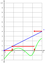
For example, the following function which composes an ODE and a discrete-time computation is correct. The value of x is added to that of o at every instant where tick is present. Between ticks, o is unchanged.
let hybrid correct(tick) = o where
  rec der x = 1.0 init 0.0
  and present tick -> do o = last o +. x done
  and init o = 0.0
The input tick has type zero, the type of zero-crossing events which are explained in the next section. The interpretation of this program is sketched in figure 2.2. The instants of activation of tick are generated (elsewhere) by monitoring a continuous expression. The value of o (in red) is recalculated at these instants by sampling the value at x and adding it onto the previous value, it is otherwise unchanged (that is, piecewise constant).
A formal presentation of the typing rules described in this section is available [2].
2.2.2 Zero-crossing Events
Zero-crossings are a standard mechanism used by numeric solvers to detect significant events. A solver recalculates the values of a set of zero-crossing expressions at each new approximation of the continuous state of a system. When one of the expressions changes sign between two successive approximations, the solver iterates to try to pinpoint the instant when the expression is equal to zero.
In Zélus, a zero-crossing expression is declared by the operator up(e). The language runtime detects when the value of the expression e changes from a negative value to a positive one during integration. The resulting events can be used to reset ODEs as illustrated in the following, classic example of a bouncing ball.
Consider a ball with initial position (x0, y0) and initial speed (x′0, y′0). Every time the ball hits the ground, it bounces but looses 20% of its speed. An example trajectory is depicted in figure 2.3.
The source program is shown below. This version is slightly simplified compared to the version giving rise to figure 2.3: the steps are not modeled and we consider that the ground is at y=0. We will reconsider this detail when we reprogram the example in section 2.3.
let g = 9.81
let loose = 0.8
let hybrid bouncing(x0,y0,x'0,y'0) = (x,y) where
 rec der x = x' init x0
 and der x' = 0.0 init x'0
 and der y = y' init y0
 and der y' = -. g init y'0 reset up(-. y) -> -. loose *. last y'
The ODE defining y’ is reset every time -.y crosses zero. At this precise instant, the initial value of y’ is -. loose *. last y’. Exactly as in chapter 1, last y’ is the value of y’ at the previous instant. But the notion of previous instant for a continuous-time signal requires clarification. Mathematically, at the instant of a reset, we need to distinguish the value of y’ just before the reset and the new value that y’ takes at the instant of the reset. As y’ is a continuous-time signal, last y’ is the left limit of y’. It corresponds to the value of y’ computed during the integration process just preceding the discrete reaction that resets y’.
Replacing last y’ by y’ leads to an error of causality. Indeed, the current value of y’ would then depend instantaneously on itself. The compiler statically rejects such programs:
let hybrid bouncing(x0,y0,x'0,y'0) = (x,y) where
 rec der x = x' init x0
 and der x' = 0.0 init x'0
 and der y = y' init y0
 and der y' = -. g init y'0 reset up(-. y) -> -. loose *. y'
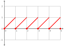
The sawtooth signal shown in figure 2.4 is another example of an ODE with reset. The signal x: ℝ+ ↦ ℝ+ is defined such that dx/dt(t) = 1 and x(t) = 0 if t∈ℕ, or as a hybrid node:
let hybrid sawtooth() = x where
  rec der x = 1.0 init 0.0 reset up(last x -. 1.0) -> 0.0
Each time last x -. 1.0 crosses zero from a negative to positive value, x is reset to zero. Note also the use of last to break what would otherwise be an invalid causality cycle.
2.2.3 Periodic Timers
A particular form of zero-crossings is provided to model timers. A timer with phase phase and period p generates an event at every instant where t = phase + n · period with n ∈ ℕ+. While such timers can be expressed directly using the features described in the previous two sections,
let hybrid timer(phase, p) = z where
  rec der t = 1.0 init -. phase reset z -> -. p
  and z = up(last t)
Zélus also provides a special period operator, which, for the moment at least, is restricted to timers of constant phase and period. For example, for a timer with phase = 10.3 and p = 20.5 one can write period 10.3(20.5). Such timers are not realized using zero-crossings, but rather by a dedicated and more efficient mechanism. At every discrete transition, the minimal ‘next value’ of all timers is computed to define the next integration horizon.
2.3 Hierarchical Automata and ODEs
We now illustrate how to combine ODEs with hierarchical automata using as an example, an hysteresis controller for a heater. We will first consider the heater dynamics. It has two modes: when active is true, the temperature increases; when active is false, it decreases. The hysteresis controller also has two modes. In the Idle mode, it outputs active = false until the temperature temp reaches the lower threshold t_min. The controller then stays in the Active mode until temp reaches the upper threshold t_max. The complete system is obtained by composing the heater and controller in parallel. Observe that the boolean signal active only changes when a zero-crossing occurs. This is a property guaranteed by the type system for all discrete (non-float) data types.
let c = 1.0
let k = 1.0
let temp0 = 0.0
let t_min = 0.0
let t_max = 1.0
(* an hysteresis controller for a heater: [c] and [k] are constant. *)
let hybrid heater(active) = temp where
  rec der temp = if active then c -. k *. temp else -. k *. temp init temp0

let hybrid hysteresis_controller(temp) = active where
  rec automaton
      | Idle -> do active = false until (up(t_min -. temp)) then Active
      | Active -> do active = true until (up(temp -. t_max)) then Idle

let hybrid main() = temp where
  rec active = hysteresis_controller(temp)
  and temp = heater(active)
The biggest difference between the automaton in the program above and those of previous programs is in the transition guards. The transition conditions of automata in a continuous context—that is, of kind C—may be either signal patterns, as described in section 1.4.11, or zero-crossing expressions, as in the example above. Notably, however, they may not be boolean expressions, though boolean expressions may still be combined with signal patterns. The equations within mode bodies inherit the kind of the automaton. In this example, we simply define active using constant expressions, but it would also have been possible to define signals by their derivatives (using der).
As always (continuous) automata may be nested hierarchically and composed in parallel. The extra structure is compiled away to generate a function that computes the temperature temp in tandem with a numeric solver and that monitors the active zero-crossing expression. The type system for automata [3] guarantees that mode changes will only occur at discrete instants, that is, in response to zero-crossing or timer events.
The ability to program with both automata and ODEs gives a restricted form of the hybrid automata of Maler, Manna, and Pnueli [15]. In particular, hybrid automata in Zélus are deterministic:
- When several transitions can be fired, for example because several conditions are true, the first one in order is taken.
- It is not possible to associate an invariant with a state. The current state is exited when a condition on an outgoing transition fires.
We will present a slightly more complicated hybrid automata by returning to the bouncing ball example of section 2.2.2. First we reprogram the vertical dynamics of the ball, this time using an external function, World.ground(), to retrieve the height of the ground as a function of the horizontal position.
(* [World.ground(x)] returns the position in [y] *)

let x_0 = 0.0
let y_0 = 8.0
let x_v = 0.72
let g = 9.81
let loose = 0.8

(* The bouncing ball *)
let atomic hybrid ball(x, y_0) = (y, y_v, z) where
  rec der y = y_v init y_0
  and der y_v = -. g init 0.0 reset z -> (-. loose *. last y_v)
  and z = up(World.ground(x) -. y)
We now incorporate these dynamics into an automaton with two modes. In Bouncing, it behaves as explained previously but for two details. When the velocity of the ball drops below a certain threshold, the system enters a Sliding mode and we gradually reduce the horizontal velocity. When Sliding, the ball only moves in the vertical dimension, until it reaches the edge of a step (as determined by a World.ground_abs() function).
let eps = 0.01

hybrid ball_with_modes(x_0, y_0) = (x, y) where
  rec init y_start = y_0
  and der x = x' init x_0
  and
  automaton
  | Bouncing ->
      (* the ball is falling with a possible bounce. *)
      local z, y_v in
      do
        (y, y_v, z) = ball(x, y_start)
      and x' = x_v until z on (y_v < eps) then Sliding(World.ground_abs(x),
                                                       World.ground(x))
  | Sliding(x0, y0) ->
      (* the ball is fixed, i.e., the derivative for y is 0 *)
      do
        y = y0
      and der x' = -0.8 *. x'
      until up(x -. x0) then do y_start = y in Bouncing
  end
This example demonstrates the hierarchical instantiation of hybrid nodes, the use of local variables in modes, shared variable resets on transition actions (...then do y_start = 0.0 in...) and a new on operator of type zero * bool -> zero which combines zero-crossing expressions and boolean conditions. The on operator emits an event when the zero-crossing occurs and the condition evaluates to true at that instant.
Futher examples are available online and in published papers [6].
Chapter 3 Compilation and Simulation
This chapter explains the basic principles behind the compilation and execution of Zélus programs. Understanding these details is useful for linking Zélus and OCaml code, either by importing OCaml values into Zélus or by exporting compiled Zélus code into OCaml.
3.1 Combinatorial Functions
Combinatorial functions are defined by the form:
They are compiled directly into OCaml functions without any particular
transformations.
3.2 Sequential Nodes
Synchronous, possibly stateful, functions are defined by the form:
They are translated as follows:
- A record type ident is introduced to represent the current value of the node’s internal state. Such records contains fields for each unit delay and -> within the node, and also for every other node instantiated within it. Values of this type are thus trees of nested records that reflect the structure of instantiations.
- A step function ident_step is introduced. Calling ident_step self pattern, where self is the current state of the node (of type ident) and pattern passes the current value of the input, returns the current output of the node and directly updates the state record self.
- A reset function ident_reset is also introduced. Calling ident_reset self resets the state self to its initial value.
- Finally, there is also an allocation function ident_alloc () which returns an initial state (of type ident).
3.3 Hybrid Nodes and Interaction with a Solver
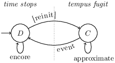
Hybrid nodes are also compiled into several functions. Their execution requires run-time support to coordinate phases of integration by a numeric solver with the execution of discrete reactions. Before outlining the form of compilation, we describe the principles behind the simulation loop provided by the run-time.
The simulation loop of a hybrid system can be formalized as a synchronous function that defines four streams lx(n), y(n), z(n) and t(n), with n ∈ ℕ. Here, t(n) is the increasing sequence of simulation times at which the solver stops;1 lx(n) is the value at time t(n) ∈ ℝ of the continuous state variables, that is, the variables defined by their derivatives in the original model; y(n) is the value at time t(n) of the model’s discrete state; and z(n) signals any zero-crossings occurring at instant t(n).
The simulation loop function has two modes: discrete (D) and continuous (C). The two modes and the transitions between them are sketched in figure 3.1. The function begins in D, where all computations that may change the discrete state or that have side effects are executed. Several discrete steps may be executed without advancing the simulation time t in what is termed an event cascade. Simulation time is advanced in C where a numeric solver is invoked to approximate the values of ODEs within the model. The function loops back to the D mode whenever a zero-crossing occurs (section 2.2.2) or a timer horizon (section 2.2.3) is reached. We now formalize the details of the two modes.
The Continuous Mode (C)
In the continuous mode C, a numeric solver computes an approximation of the solution of the set of (active) ODEs within a model. We represent the solver abstractly as a function solve(f)(g) parameterized by two other functions f and g:
- x′(τ) = f(y(n), τ, x(τ)) yields the derivatives of continuous state variables x at τ ∈ ℝ, given the discrete states y(n) and an approximation to the continuous states x(τ);
- upz(τ) = g(y(n), τ, x(τ)) computes the value of the zero-crossing expressions upz given the same arguments as f.
For a given f and g, the continuous mode C computes s, lx, z, and t such that:
| (lx, z, t, s)(n+1) = solve(f)(g)(s, y, lx, t, step)(n) |
where
- s(n)
- is the internal state of the solver at instant t(n) ∈ ℝ. Calling solve(f)(g) updates the state to s(n+1).
- lx(n)
- is the value of x at instant t(n), that is, lx(n) = x(t(n)); lx is a discrete-time signal while x is a continuous-time signal.
- t(n+1)
-
is bounded by the horizon given to the solver t(n) + step(n), that is,
t(n) ≤ t(n+1) ≤ t(n) + step(n) - x
-
is a solution of an ODE, parameterized by the current discrete state y(n),
that is:
Integration is performed on an interval strictly larger than [t(n),t(n+1)] to account for possible zero-crossings at instant t(n+1). The constant margin is considered as a parameter of the solver. In practice, solve(f)(g) computes a finite sample of approximated values on the interval [t(n), t(n+1) + margin]. The value of lx(n+1) is∀ T ∈ [t(n), t(n+1) + margin] x(T) = lx(n) + ∫ T
t(n) f (y(n), τ, x(τ))) dτ lx(n+1) = x(t(n+1)) - z(n+1)
-
signals any zero-crossings detected at time t(n+1).
It comprises k ∈ ℕ boolean elements z(n+1)(i) such that:
This definition assumes that the solver also stops whenever a zero-crossing expression passes through zero from positive to negative. An event occurs with a transition to the discrete phase (D) when a zero-crossing occurs or the horizon t(n)+step(n) is reached:z(n+1)(i) = (∀ T ∈ ⎡
⎣t(n), t(n+1) ⎞
⎠upz(T)(i) < 0) ∧ ∃ m ≤ margin. (∀ T ∈ [t(n+1), t(n+1)+m] upz(T)(i) ≥ 0) event = z(n+1)(0) ∨ … ∨ z(n+1)(k) ∨ t(n+1) = t(n) + step(n)
If the solver raises an error (for example, a division by zero occurs, or a suitable approximation cannot be found), we consider that the simulation fails.
The Discrete Mode (D)
All discrete changes occur in this mode. It is entered when an event occurs during integration. During a discrete phase, the function next defines y, lx, step, encore, z, and t:
|
where:
- y(n+1)
- is the new discrete state (outside of mode D, y(n+1) = y(n));
- lx(n+1)
- is the new continuous state, which may be directly changed in the discrete mode;
- step(n+1)
- is the new step size;
- encore(n+1)
- is true if an additional discrete step must be performed. Function next can decide to trigger another discrete event instantaneously causing an event cascade.
- t(n)
- (the simulation time) is unchanged during a discrete phase.
The initial values for y(0), lx(0) and s(0) are given by an initialization function init. Finally, solve(f)(g) may decide to reset its internal state when the continuous state changes. If init_solve(lx(n), s(n)) initializes the solver state, then we have:
|
These definitions give a synchronous interpretation of the simulation loop, seen as a stream function that iteratively computes the sequences lx, y and t at instant n+1 relative to their values at instant n and an internal state. By writing solve(f)(g), we abstract the actual choices of the integration method and zero-crossing detection algorithms. A more detailed description of solve(f)(g) would be possible (for example, as an automaton with two states: one that integrates, one that detects zero-crossings) but these details have no influence on the code generation problem which is independent of such simulation details.
Hybrid functions are defined by the form:
They are compiled into six functions:
- A record type ident is introduced to represent the current value of the function’s internal state. In addition to fields for each unit delay, -> operator, and node instantiation within the function body, it also contains fields for continuous state variables (those defined with der) and zero-crossing expressions (those registered with up()).
- A step function ident_step is introduced. Calling ident_step self pattern, where self is the current state of the node (of type ident) and pattern passes the current value of the input, returns the current output of the node and directly updates the state record self.
- The abstract function f, in the above formalization, is realized by the function ident_derivatives self pattern that computes the current values of derivatives from the current state and stores them in the internal state self.
- The abstract function g, in the above formalization, is realized by the function ident_crossings self pattern that computes the current values of zero-crossing expressions and stores them in the internal state self.
- A reset function ident_reset is also introduced. Calling ident_reset self resets the state self to its initial value.
- Finally, there is also an allocation function ident_alloc () which returns an initial state (of type ident).
- 1
- They are called major time steps in Simulink.
Part II |
Chapter 4 The language
The syntax of the language is presented in BNF-like notation. Terminal symbols are set in typewriter font (like this). Non-terminal symbols are set in italic font (like that). Square brackets [ ... ] denote optional components. Curly brackets { ... } denotes zero, one, or several repetitions of the enclosed components.
4.1 Lexical conventions
We adopt the lexical conventions of OCaml for blanks, comments, identifiers, integer literals, floating-point literals, character literals, string literals, and prefix and infix symbols.
Keywords
The following identifiers are reserved as keywords.
  as      automaton  atomic   inline  continue  disc  do    done   until
  unless  emit       present  match   period    with  end   fun    node
  hybrid  discrete   init     in      and       open  val   local  unsafe
  let     rec        where    open    fby       next  up    der    reset
  pre     type       every    true    false     or    on    last   if
  then    else       quo      mod     land      lor   lxor  lsl    lsr
  asr
The following character sequences are also keywords.
        ->   >     <     =     <>     >=        )     &  ?
        +    -     *     /     ;;     <=        (     .
4.2 Values
4.2.1 Basic values
Zélus provides the basic values of OCaml—that is, integer numbers, floating-point numbers, characters and character strings—and with the same conventions.
4.2.2 Tuples, records, sum types
Zélus provides the tuples of OCamlwith the same conventions. It also provides records and sum types with constructors of arity 0.
Functions
Functions map values to other values. They are separated into three main categories: pure or combinatorial functions, discrete-time stateful functions, and continuous-time stateful functions.
4.3 Global names
The naming conventions in Zélus are inherited from OCamlsubject to the restrictions detailed in this section.
Names in Zélus fall into one of three syntactic classes:
- value-name for value names,
- typeconstr-name for type constructors, and
- module-name for module names.
4.3.1 Naming values
| value-name | ::= | lowercase-ident |
| | | ( operator-name ) | |
| operator-name | ::= | prefix-symbol | infix-symbol | * | = | or | & | || |
| constructor-name | ::= | capitalized-ident |
| | | () | |
| typeconstr-name | ::= | lowercase-ident |
| module-name | ::= | capitalized-ident |
The syntactic class of lowercase-ident is the set of identifiers starting with a lowercase letter whereas capitalized-ident is the set of of identifiers starting with a capital letter.
4.3.2 Referring to named values
| value-path | ::= | value-name |
| | | module-name . value-name | |
| constructor | ::= | constructor-name |
| | | module-name . capitalized-ident | |
| typeconstr | ::= | typeconstr-name |
| | | module-name . typeconstr |
A value can be referred to either by its name or by its name qualified with a module name.
4.4 Types
| type | ::= | ’ ident |
| | | ( type ) | |
| | | type {* type} | |
| | | type typeconstr | |
| | | ( type {, type }) typeconstr | |
| | | typeconstr |
| ftype | ::= | type -> type |
4.5 Constants
| immediate | ::= | integer-literal |
| | | float-literal | |
| | | char-literal | |
| | | string-literal | |
| | | boolean-literal |
Constants are formed of literals from the base types (integers, floating-point numbers, characters, character strings, and booleans).
4.6 Patterns
Patterns allow binding identifiers to the components of data structures.
| pattern | ::= | ident |
| | | ( pattern ) | |
| | | pattern as ident | |
| | | _ | |
| | | pattern , pattern { , pattern } | |
| | | () | |
| | | immediate | |
| | | constructor | |
| | | { label = pattern { ; label = pattern } } |
4.7 Signal Patterns
Signal patterns allows for testing the presence of signals and for binding their values with patterns. A boolean expressions is also considered a signal pattern (in non-continuous contexts).
| signal-pattern | ::= | simple-expr |
| | | simple-expression pattern | |
| | | signal-pattern on simple-expr | |
| | | signal-pattern & signal-pattern | |
| | | signal-pattern || signal-pattern |
4.8 Expressions
| simple-expr | ::= | value-path |
| | | constructor | |
| | | immediate | |
| | | ( expr ) | |
| | | { label = expr { ; label = expr } } | |
| | | simple-expr . label | |
| pattern-list | ::= | pattern { pattern } |
| expr | ::= | simple-expr |
| | | value-path simple-expr | |
| | | let [ rec ] definition { and definition } in expr | |
| | | if expr then expr else expr | |
| | | prefix-op expr | |
| | | expr infix-op expr | |
| | | up expr | |
| | | not expr | |
| | | expr fby expr | |
| | | pre expr | |
| | | expr -> expr | |
| | | last ident | |
| | | match expr with match-handlers [ end ] | |
| | | reset expr every expr | |
| | | present present-handlers [ end ] | |
| infix-op | ::= | infix-symbol | * | = | or | || | & |
| match-handlers | ::= | [ | ] pattern -> expr { | pattern -> expr } |
| present-handlers | ::= | [ | ] signal-pattern -> expr { | signal-pattern -> expr } |
The precedence and associativity rules of OCamlare adopted. The rules for Zélus-specific primitives are, in order from highest to lowest precedence:
| last | right |
| pre | - |
| function application | - |
| fby | left |
| ... let,... | - |
| -> | right |
4.8.1 Simple expressions
Constants
A constant expression, like 1 or false, denotes an infinite stream of that constant.
Variables
A variable evaluates to the value bound to that variable in the current evaluation environment.
Parenthesized expressions
The expression ( expr ) has the same value as expr.
Local definitions
The let and let rec constructs bind variables locally. The expression
defines values to be visible in expr. In a let definition, variables names appearing on the right of an equality are bound to their definition in the current environment. This environment does not contains names from the let definition itself.
Recursive definitions of variables are introduced by let rec:
In a recursive definition the current environment also contains names defined within the let construction itself.
4.8.2 Operators
The operators written infix-op in the grammar are applied by placing them between two expressions. The operators written prefix-op in the grammar are applied by placing them in front of an expression.
The basic operators provided by OCaml (from the Pervasives module) are imported. Scalar values imported from the host language become stream operators that are applied pointwise.
Unit Delays
The expression pre expr denotes the delayed stream. The nth value of the result is the n−1th value of expr. The value at the first instant is undefined.
The binary operator fby is the initialized delay operator. The first value of expr1 fby expr2 is the first value of expr1. The nth value is the n−1th value of expr2.
These two delay operators may only be activated on a discrete clock. In Zélus (version 1.2) this is ensured by imposing that they appear only in contexts of kind k = D.
Initialization Operation
The expression expr1 -> expr2 initializes a stream. The expri must be streams of the same type. The first value of the result is the first value of expr1, after which the nth value of the result is the nth value of expr2.
The initialization operator must be activated on a discrete clock.
Access to a Shared State Variable
The expression last ident denotes the previous computed value of the variable ident.
As opposed to the unit delays, pre and fby, the operator last only applies to variable names and it can be activated on both discrete and continuous clocks. Nonetheless, when last x appears in a continuous context, Zélus (version 1.2) imposes that x be a continuous state variable; in other words, it must be defined directly by an equation of the form der x = e.
Point-wise conditional
The expression if expr1 then expr2 else expr3 is the pointwise conditional: expr1 must be a boolean stream and expr2 and expr3 must be two streams of the same type. The type of the result is the type of expr2.
Warning: this operator is strict, that is, at every step, both branches are evaluated regardless of the value of the condition. The result at instant n is the value of expr2 if the value of expr1 is true and the value of expr3 otherwise.
Function application
The expression value-path simple-expr is the application of the function value-path to the expression simple-expr.
4.8.3 Control Structures
The constructions reset, match/with, reset, and automaton are control-structures which combine equations and thus belong to the syntactic class of definitions (see section 4.9).
A derived form belonging to the syntactic class of expressions is also provided. The derived form is useful for textual programming whereas the original one is motivated by the graphical representation of dataflow programs. The derived form is only syntactic sugar for the original form.
Pattern Matching over Expressions
The expression match expr with pat1 -> expr1 | …| patn -> exprn end is a short-cut for the expression:
| let | match expr with |
| | pat1 -> do o = expr1 done | |
| … | |
| | patn -> do o = exprn done | |
| end in | |
| o |
provided that o is a fresh name.
Modular Reset over Expressions
The expression reset expr1 every expr2 is a short-cut for let reset o = expr1 every expr2 in o, provided that o is a fresh name.
Automata
The expression automaton state1 -> expr1 trans1 | …| staten -> exprn transn end is a short-cut for the expression:
| let | automaton |
| | state1 -> do o = expr1 trans1 | |
| … | |
| | staten -> do o = exprn transn | |
| end in | |
| o |
provided that o is a fresh name.
Testing Presence
The expression present spat1 -> expr1 | …| spatn -> exprn end is a short-cut for the expression:
| let | present |
| | spat1 -> do o = expr1 done | |
| … | |
| | spatn -> do o = exprn done | |
| end in | |
| o |
provided that o is a fresh name.
4.9 Definitions
| value-definition | ::= | let ident = expr |
| | | [ let ] [ kind ] ident pattern = result-expr | |
| function-kind | ::= | fun | node | hybrid |
| result-expr | ::= | expr [ where [ rec ] definition { and definition } ] |
| definition | ::= | pattern = expr |
| | | init ident = expr | |
| | | emit ident = expr | |
| | | match expr with def-match-handlers [ end ] | |
| | | reset definition { and definition } every expr | |
| | | automaton def-automaton-handlers [ end ] | |
| | | present def-present-handlers [ else definition ] [ end ] | |
| | | [ local-definitions ] do definition-list done | |
| definition-list | ::= | [ definition { and definition } ] |
| local-definitions | ::= | { let [ rec ] definition { and definition } in } { local ident in } |
Global Value Definition
A global definition ident = expr defines the value of the global identifier ident to be equal to the value of expr in the current global environment. The expression expr must be combinatorial.
Global Function Definition
A global function definition is of the form:
with
| function-kind | ::= | fun | node | hybrid |
where
- fun is the kind of combinatorial functions—typically a function imported from the host language and applied pointwise. Its body result-expr must only contain combinatorial operations. In particular, it may not invoke stateful functions like unit delays or integrators.
- node is the kind of (possibly) stateful discrete-time functions—typically a synchronous function that must be activated on a discrete-time scale. Its body result-expr must only contain combinatorial and discrete-time stateful operations. In particular, it may not invoke continuous-time operators like integrators or zero-crossing detection.
- hybrid is the kind of (possibly) stateful continuous-time functions—typically a function that contains ODEs and/or zero-crossing detection and must be activated continuously. It may contain all kinds of operator provided that discrete-time operations are activated on discrete events.
Alternative Syntax for Local Definitions
The language provides an alternate form of local definitions for returning the results of functions. The expression:
has the meaning of:
Equation
The equation pattern = expr defines the current value of pattern to be equal to the current value of expr.
Initialization of a State Variable
A definition init ident = expr initializes the value of last ident with the value of expr.
Signal Emission
An equation emit ident = expr defines the signal ident to be equal to the value of expr. At every instant, a signal can be absent or present. When present, it carries a value.
Pattern Matching
| def-match-handlers | ::= | [ | ] def-match-handler { | def-match-handler } |
| def-match-handler | ::= | pattern -> definition |
The construct match expr with pattern1 -> action1 | ... | patternn -> actionn end is used to combine n complementary sub-streams. Each of these streams is on the clock defined by the instants where the value of e has the form patterni .
Each definition can define local and shared variables. Shared variables are variables that may be defined and used across several branches and which are not bound by a local construct.
Reinitialization
The construct reset definition1 and ... and definitionn every expr allows for resetting the computation defined by a set of definitions. All the defined values and expression expr must be on the same clock. This construction acts as a regular multi-definition except that the streams and automata defined in definition1,..., definitionn restart with their initial values every time the current value of expr is true. In particular, automata appearing in definition1,..., definitionn restart in their initial states.
Hierarchical Automata
| def-automaton-handlers | ::= | [ | ] def-automaton-handler { | def-automaton-handler } |
| def-automaton-handler | ::= | constructor [ pattern ] -> automaton-definition |
| automaton-definition | ::= | local-definitions do definition-list transitions |
| transitions | ::= | done |
| | | then state-expression | |
| | | continue state-expression | |
| | | unless transition { else transition } | |
| | | until transition { else transition } | |
| transition | | | signal-pattern then [ local-definitions do definition-list ] in state |
| | | signal-pattern continue [ local-definitions do definition-list ] in state | |
| state-expression | ::= | constructor |
| | | constructor ( expr ) |
The construction automaton def-automaton-handler | ... | def-automaton-handler end defines an automaton. Each branch of the automaton has either the form:
or the form
where constructor denotes the name of the state. This state may be parameterized by a pattern. The first branch defines the initial state and this state cannot be parameterized unless an initialization clause is given.
The action associated to a state has the form:
It comprises a (possibly empty) sequence of local definitions to the state, a definition list of shared variables, and a (possibly empty) list of transitions to be tested sequentially. Transitions may have several forms. Writing:
defines a weak transition which is executed within the current reaction but at the end of it, that is, after definitions from the current state have been executed. Transitions are all evaluated in the same instant but sequentially: the first transition to succeed determines the target state at the next reaction. Writing:
defines a strong transition which is executed before the reaction starts, that is, before definitions from the current state have been executed. Transitions are all evaluated in the same instant but sequentially: the first transition to succeed determines the current active state.
A transition may reset or not the history of the state being entered. Writing:
indicates that the target state is entered by reset, that is, all streams and automata in the target state restart with their initial values. Writing:
has the same behavior except that the target state is entered by history, that is, no reset occurs. For both kinds of transition (reset or history), the condition signal-pattern is tested. When it is true, local-definitions do definition-list in state are executed in the same reaction.
The language provides two transition shorthands:
- The transition then state is shorthand for until true then state
- The transition continue state is shorthand for until true continue state.
Zélus (version 1.2) forbids the mixing of weak and strong conditions within a single automaton (not counting nested automata). This differs from Lucid Synchrone, for example, which allows for arbitrary combinations within an automaton. We made this choice to simplify code generation and allow for more efficient execution. But we may lift this restriction in a future release.
Testing the Presence of a Signal
The present construct resembles the pattern-matching one. It has the form:
where a handler has the form:
| def-present-handlers | ::= | [ | ] def-present-handler { | def-present-handler } |
| def-present-handler | ::= | signal-pattern -> definition |
At every instant, signal patterns are tested sequentially and the one which first succeeds determines the action to execute. The optional handler:
defines a condition which always succeed and thus gives a default action.
4.10 Type definition
Abstract types can be defined. Their syntax is inherited from OCaml and recalled here.
| type-definition | ::= | type typedef { and typedef } |
| typedef | ::= | [ type-params ] typeconstr-name |
| | | sum-type-def | |
| | | record-type-def | |
| sum-type-def | ::= | [ | ] one-sum-def { | one-sum-def } |
| one-sum-def | ::= | capitalized-ident |
| record-type-def | ::= | { label-type { ; label-type } } |
| label-type | ::= | ident : type |
| type-params | ::= | ’ ident |
| | | ( ’ ident { , ’ ident } ) |
4.11 Module implementation
| implementation | ::= | { impl-phrase [ ;; ] } |
| impl-phrase | ::= | value-definition |
| | | type-definition | |
| | | open module-name |
A module implementation comprises a sequence of implementation phrases. An implementation phrase either opens a module, declares a type, or defines a sequence of values.
- The instruction open modifies the list of opened modules by adding the module name to the head of the list of opened modules.
- The type definition defines a type from the implementation phrases following the definition.
- The value definition defines global values.
4.12 Importing values
Scalar interfaces written in OCaml can be imported into Zélus. In the current implementation, a restricted subset of OCaml interfaces is considered. The syntax is the following:
| scalar-interface | :: = | { scalar-interface-phrase [ ;; ] } |
| scalar-interface-phrase | ::= | value-declaration |
| | | type-definition | |
| value-declaration | ::= | val ident : type |
When a value is imported from OCaml, it is automatically lifted to the stream level:
- A scalar value with a basic or declared type becomes an infinite stream of that type.
- A scalar functional value becomes a stream functional value applied pointwise to its argument.
Chapter 5 zeluc
The Zélus compiler is called zeluc. Given a list of options and a filename, it transforms Zélus source code into OCaml source code.
zeluc [option] filename
where options are:
  -v             Set verbose mode
  -version       The version of the compiler
  -I <dir>       Add <dir> to the list of include directories
  -i             Print types
  -ic            Print causality types
  -where         Locate standard libray
  -stdlib <dir>  Directory for the standard library
  -nopervasives  Do not load the pervasives module
  -typeonly      Stop after typing
  -s <node>      Simulates the node <node> and generates a file <node>.ml
                 For hybrid programs, compile with:
                 bigarray.cma unix.cma -I +sundials sundials_cvode.cma zllib.cma
  -sampling <p>  Sets the sampling period to p (float <= 1.0)
  -check <n>     Check that the simulated node returns true for n steps
  -gtk2          Use lablgtk2 interface.
                 Compile with: -I +lablgtk2 lablgtk.cma zllibgtk.cma
  -dzero         Turn on discrete zero-crossing detection
  -nocausality   (undocumented)
  -noinit        (undocumented)
  -inline <n>    Level of inlining
  -help          Display this list of options
  --help         Display this list of options
Three kinds of arguments are accepted:
-
Arguments ending in
.zlsare interpreted as Zélus source files. These files must contain sequences of node declarations. The zeluc compiler turns.zlsfiles into a compiled interfacef.zciand an OCaml filef.ml. The.mlfile defines the corresponding transition functions for the values defined in the input file. - Arguments ending in
.zliare interpreted as Zélus interface files. These files define type signatures for values implemented elsewhere. The zeluc compiler turns.zlifiles into a compiled interfacef.zci. - Arguments ending in
.mliare interpreted as OCaml interface files. The zeluc compiler turns.mlifiles into a compiled interfacef.zci. The values defined inf.mliare considered to be a scalars.
SEE ALSO
The distribution and manual are available at http://zelus.di.ens.fr.
FILES
| /usr/local/bin/zeluc | the compiler |
| /usr/local/lib/zeluc | the standard library |
References
- [1]
- E. A. Ashcroft and W. W. Wadge. Lucid, a non procedural language with iteration. Communications of the ACM, 20(7):519–526, 1977.
- [2]
- A. Benveniste, T. Bourke, B. Caillaud, and M. Pouzet. Divide and recycle: types and compilation for a hybrid synchronous language. In ACM SIGPLAN/SIGBED Conference on Languages, Compilers, Tools and Theory for Embedded Systems (LCTES’11), Chicago, USA, April 2011.
- [3]
- A. Benveniste, T. Bourke, B. Caillaud, and M. Pouzet. A hybrid synchronous language with hierarchical automata: Static typing and translation to synchronous code. In ACM SIGPLAN/SIGBED Conference on Embedded Software (EMSOFT’11), Taipei, Taiwan, October 2011.
- [4]
- A. Benveniste, P. LeGuernic, and Ch. Jacquemot. Synchronous programming with events and relations: the SIGNAL language and its semantics. Science of Computer Programming, 16:103–149, 1991.
- [5]
- G. Berry. The Esterel v5 language primer, version 5.21 release 2.0. Draft book, 1999.
- [6]
- T. Bourke and M. Pouzet. Zélus, a Synchronous Language with ODEs. In International Conference on Hybrid Systems: Computation and Control (HSCC 2013), Philadelphia, USA, April 2013. ACM.
- [7]
- Timothy Bourke and Arcot Sowmya. Delays in Esterel. In Albert Benveniste, Stephen A. Edwards, Edward Lee, Klaus Schneider, and Reinhard von Hanxleden, editors, 16th Open International Workshop on Synchrononous Programming (SYNCHRON 2009), number 09481 in Dagstuhl Seminar Proceedings, pages 55–84, Dagstuhl, Germany, 2010. Schloss Dagstuhl - Leibniz-Zentrum für Informatik, Germany.
- [8]
- P. Caspi, G. Hamon, and M. Pouzet. Modeling and Verification of Real-Time Systems: Formalisms and Software Tools, chapter Synchronous Functional Programming with Lucid Synchrone. ISTE Ltd, 2007.
- [9]
- J.-L. Colaço, B. Pagano, and M. Pouzet. A conservative extension of synchronous data-flow with state machines. In ACM International Conference on Embedded Software (EMSOFT’05), Jersey city, New Jersey, USA, September 2005.
- [10]
- J.-L. Colaço and M. Pouzet. Type-based initialization analysis of a synchronous data-flow language. International Journal on Software Tools for Technology Transfer (STTT), 6(3):245–255, August 2004.
- [11]
- G. Dahlquist and Å. Björck. Numerical Methods in Scientific Computing: Volume 1. SIAM, 2008.
- [12]
- N. Halbwachs, P. Caspi, P. Raymond, and D. Pilaud. The synchronous dataflow programming language Lustre. Proceedings of the IEEE, 79(9):1305–1320, September 1991.
- [13]
- A. C. Hindmarsh, P. N. Brown, K. E. Grant, S. L. Lee, R. Serban, D. E. Shumaker, and C. S. Woodward. SUNDIALS: Suite of nonlinear and differential/algebraic equation solvers. ACM Transactions on Mathematical Software, 31(3):363–396, September 2005.
- [14]
- R. Lublinerman, C. Szegedy, and S. Tripakis. Modular code generation from synchronous block diagrams—modularity vs. code size. In ACM Principles of Programming Languages (POPL), 2009.
- [15]
- O. Maler, Z. Manna, and A. Pnueli. From timed to hybrid systems. In Real-Time: Theory in Practice, volume 600 of LNCS, pages 447–484. Springer, 1992.
- [16]
- F. Maraninchi and Y. Rémond. Mode-automata: a new domain-specific construct for the development of safe critical systems. Science of Computer Programming, 46:219–254, 2003.
- [17]
- M. Pouzet and P. Raymond. Modular static scheduling of synchronous data-flow networks: An efficient symbolic representation. In ACM International Conference on Embedded Software (EMSOFT’09), Grenoble, France, October 2009.
- [18]
- L. F. Shampine, I. Gladwell, and S. Thompson. Solving ODEs with Matlab. Cambridge University Press, 2003.
This document was translated from LATEX by HEVEA.