A Type-based Analysis of Causality Loops in Hybrid Systems Modelers

A Miscompiled Simulink Model

This example demonstrates some subtelties in the scheduling of integrator resets with feedback. In particular, the result given by Simulink is inconsistent with its documentation.

Simulink

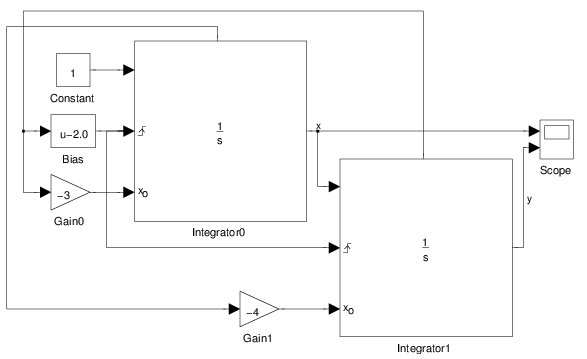
• Download the Simulink model.
• See the Simulation log.
• See the Raw results.

According to the Simulink documentation for the State port,

The output of the state port is the same as the output of the block's standard output port except for the following case. If the block is reset in the current time step, the output of the state port is the value that would have appeared at the block's standard output if the block had not been reset.

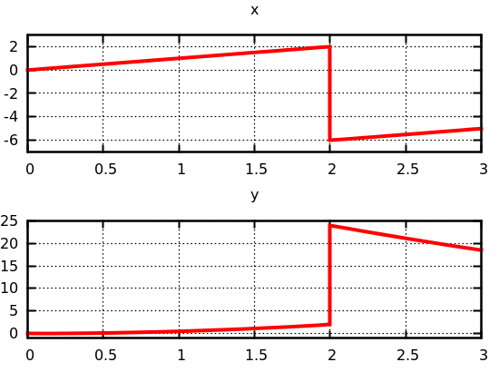
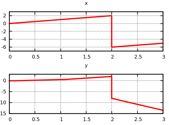
Now, in this case, the y signal should be reset to -8 at t = 2 according to the scenario:

1. Initially, both x and y are 0.
2. At t = 2, the state port of Integrator1 becomes equal to 2 which triggers resets at each integrator.
3. Integrator0 should be reset to -3 times the value of Integrator1 (y) before any reset, i.e., to -6.
4. Integrator1 should be reset to -4 times the value of Integrator0 (x) before any reset, i.e., to -8.

But, in fact, the y signal is reset to 24, i.e., -4 times the value of Integrator0 (x) after it has been reset to -6!

Zélus

The equivalent Zélus program, however, gives the expected result.

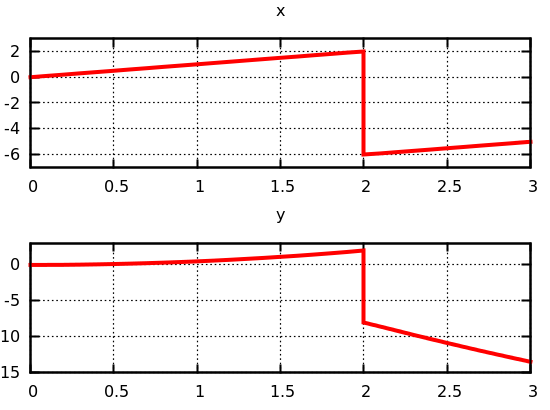
• See the Raw results.

open Dump

let node plot (t, x, y) =
  let s1 = scope (-7.0,  3.0, ("x", linear, x)) in
  let s2 = scope ( 0.0, 25.0, ("y", linear, y)) in
  window2 ("zelus", 3.0, t, s1, s2)

let hybrid main () = () where
  rec der x = 1.0 init 0.0 reset z -> -3.0 *. last y
  and der y = x   init 0.0 reset z -> -4.0 *. last x
  and z = up(last x -. 2.0)

  and der t = 1.0 init 0.0
  and present (init) | z | (period (0.1)) -> do () = plot (t, x, y) done

In the Zélus version of the Simulink model, the ‘state port’ of Integrator0 is written last(x), and the ‘state port’ of Integrator1 is written last(y).

We plot values at the initial instant, when a reset is detected, and otherwise every 0.1 seconds.

Ptolemy II

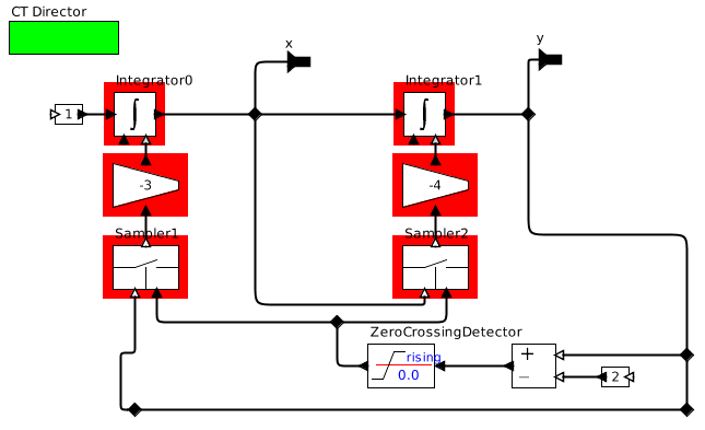
A first, naive attempt at modeling this example, fails with the error:

ptolemy.actor.sched.NotSchedulableException: Algebraic loop. Cycle includes:
.dder_loop_reset.Integrator0,
.dder_loop_reset.Scale1,
.dder_loop_reset.Sampler1,
.dder_loop_reset.Integrator1,
.dder_loop_reset.Scale2,
.dder_loop_reset.Sampler2 in
.dder_loop_reset.Integrator0,
.dder_loop_reset.Scale1,
.dder_loop_reset.Sampler1,
.dder_loop_reset.Integrator1,
.dder_loop_reset.Scale2,
.dder_loop_reset.Sampler2

The documentation explains why:

An integrator can generate an output (its current state) before the derivative input is known, and hence can be used in feedback loops like that above without creating a causality loop. The impulse and initialState inputs ports must be known, however, before an output can be produced. The effect of data at these inputs on the output is instantaneous.

In fact, the rest has to be ‘scheduled’ in super-dense time. We restart with a modal model:

where the Running state is refined by a continuous model:

The reset event is detected by a Level Crossing Detector which triggers the reset transition in the modal model (hitisPresent_). The documentation indicates that a delay is introduced by the detector:

This actor will also not produce an event if the current microstep is 0. In that case, the output is postponed by one microstep. This ensures that the output signal, which is discrete, satisfies the piecewise continuity constraint, and is absent at microstep 0.

which, in this case breaks the algebraic loop. The looping reset transition sets the values of two parameters which are used to initialize the integrators in the refinement.

This model gives the expected result:

• Download the Ptolemy model.
• See the Raw results.

A Nonsmooth Model

This example shows that, in a non-standard semantics, care must be taken to avoid introducing discontinuities that are not aligned with discrete events. The models use discrete events to produce a pulse of very short, ideally infinitesimal, duration. This pulse causes, at a later time, a ‘jump’ in the output signal.

The main idea is to model a function \(l_d(t)\), where \(d\) represents the width of an input pulse. The behaviour of the function has a discontinuity when \(d\) is a (positive) infinitesimal.

Simulink

Time always passes in Simulink and there is anyway no concrete notion of an infinitesimal value. So we model a very small (\(1\times 10^{-6}\)) pulse width.

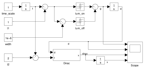
The Simulink model is very stiff at t = 0, but not discontinuous. All of its discontinuities are aligned with discrete events (zero-crossings at t = 1 and t = 1 + 1e-6).

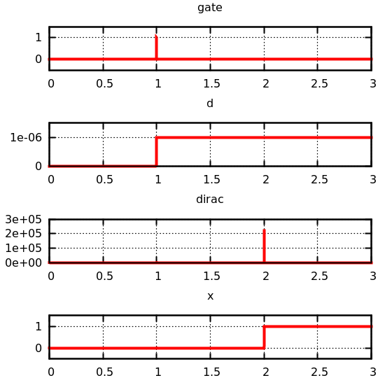
• Download the Simulink model.
• See the Simulation log.
• See the Raw results.

Zélus

Zélus has a notion of instantaneous transitions separated, in theory, by an infinitesimal. We can thus try to model a pulse of infinitesimal width.

let hybrid integrator(y0, x) = y where
  der y = x init y0

let hybrid time(t0) = integrator(t0, 1.0)

let pi = 4.0 *. (atan 1.0)

let dirac(d, t) = 1.0 /. pi *. d /. ( d *. d +. t *. t)

let hybrid doublecrossing(t) = (x +. 1.0) /. 2.0
  where
  rec init x = -1.0
  and present up(t) -> do next x =  1.0 done
            | up(x) -> do next x = -1.0 done
            else do der x = 0.0 done

let hybrid model(t0, t1, t2) = (g, i, d, x) where
  rec lt = time(t0)
  and g = doublecrossing(lt -. 1.0)
  and i = integrator(0.0, g)
  and d = dirac(i, (lt -. t2))
  and x = integrator(0.0, d)

open Dump

let t0 = 0.0
let t1 = 1.0
let t2 = 2.0

let hybrid main () = () where
  rec (g, d, x, y) = model(t0, t1, t2)
  and t = time(t0)
  and _ = present (init) | (period(0.5)) ->
            let s1 = scope(0.0, 2.0, ("gate",   points false, g))
            and s2 = scope(0.0, 2.0, ("delta",  points false, d))
            and s3 = scope(0.0, 2.0, ("dirac",  points false, x))
            and s4 = scope(0.0, 2.0, ("result", points false, y))
            in window4("zelus", 3.0, t, s1, s2, s3, s4)

The implementation is, of course, based on standard numeric solvers and not by simulation with non-standard values! Thus, even though, at t = 1, doublecrossing takes the value 1, before immediately returning to 0, its integral, i, does not advance and remains equal to 0. This means that later, at t = 2, the function dirac is not properly defined since there will be a division by zero rather than a division by a very small number.

A singularity at an instant will not necessarily be detected during numerical simulation. It depends on when the solver ‘samples’. In the above source code we set the sample time to 0.5 to ensure that the solver executes the system at t = 2. But, the argument to dirac is lt - t2 where lt is calculated within the program. Its exact value at t = 2 depends on numerical factors, like, for instance, the maximum simulation time. For instance, with maxt=2.5 at t = 2, we had lt = 2.000000000000001e+00 and no singularity. But, with maxt = 3.0 at t = 2, we had lt = 2.000000000000000e+00, for which dirac returns nan, and for which the solver then fails to converge:

[CVODE ERROR]  CVode
  At t = 2 and h = 9.78932e-11, the corrector convergence test failed repeatedly or with |h| = hmin.

Fatal error: exception Cvode.ConvergenceFailure

Miscellaneous Examples

Sawtooth signal

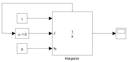
The sawtooth signal is simple to program but already raises questions of causality, since the value being defined, y, also occurs on the right-hand side of the definition as a trigger of resets.

open Dump

let hybrid main () = () where

  (* A sawtooth signal *)
  rec der y = 1.0 init 0.0 reset up(last y -. 1.0) -> 0.0

  (* Plot values of y at regular intervals *)
  and der t = 1.0 init 0.0
  and _ = present (init) | (period(0.001)) ->
            let s = scope(-1.2, 0.2, ("y", linear, y))
            in window("sawtooth", 5.0, t, s)

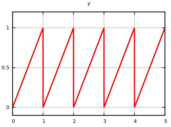
The same example is also readily programmed in Simulink with a single integrator, whose state port can be seen leaving the top of the block.

• Download the Simulink model.
• See the Simulation log.
• See the Raw results.

Integrator reset from memory

This example is similar to the previous one, but rather than detect zero-crossings on, and set the initial state of an integrator from its state port, we do so using a memory block.

The exact results depend on the steps chosen by the solver. These steps can be influenced by placing another (very simple) model in parallel. In this case, a sine wave connected to a zero-crossing detector. If the sine wave frequency is set to 0.1, we see the following:

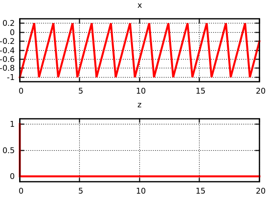
where there are 12 peaks during the simulation. If, however, the sine wave frequency is set to 10.0, we see the following:

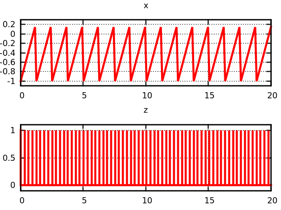
where there are 15 peaks during the simulation.

Two modes

This example shows the memory block being used to synchronize the state values of two mutually exclusive) subsystems. The main Simulink model:

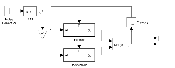
contains an enabled subsystem called ‘Up mode’:

and another called ‘Down mode’:

The pulse generator alternates between the subsystems. Each time a subsystem is enabled, its internal integrator is reset to the value at the subsystem input. This value comes from a Memory block. In this way, the integrators ‘guide’ the output signal x between -1 and 1:

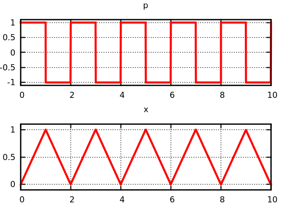
To get the ‘sharp points’ on the graph of x, we had to set the maximum simulation step to 0.01. Mode changes only occur on major time steps, which are sensitive to such parameters and also to zero-crossings. In this case, even adding a hit crossing did not help.

• Download the Simulink model.
• See the Simulation log.
• See the Raw results.