Chapter 2  Hybrid Systems Programming

In this chapter we introduce the main novelty of Zélus with respect to standard synchronous languages: all of the previously introduced constructs, that is, stream equations and hierarchical automata, can be combined with Ordinary Differential Equations (ODEs). As before, we only present basic examples in this document. More advanced examples can be found on the examples web page.

2.1  Initial Value Problems

Consider the classic Initial Value Problem that models the temperature of a boiler. The evolution of the temperature t is defined by an ODE and an initial condition:

where g₀ and g₁ are constant parameters and t₀ is the initial temperature. Instead of choosing an explicit integration scheme as in section 1.1.8, we can now just write the ODE directly:

let hybrid heater(t0, g0, g1) = t where
  rec der t = g0 -. g1 *. t init t0

The der keyword defines t by a (continuous) derivative and an initial value. Notice that the hybrid keyword is used here rather than node. It signifies the definition of a function between continuous-time signals. This is reflected in the type signature inferred by the compiler with its -C-> arrow. The C stands for “continuous” Hybrid functions need special treatment for simulation with a numeric. Discrete nodes, on the other hand, evolve in logical time, that is, as a sequence of instants, and may not contain any nested continuous-time computations.

As a second example of the new features, consider the following continuous definition of the sine and cosine signals whose stream approximation was given in section 1.1.6:

let hybrid sin_cos theta = (sin, cos) where
  rec der sin = theta *. cos init 0.0
  and der cos = -. theta *. sin init 1.0

Are these definitions really all that different from those in the previous chapter? Yes!

The dynamics of the boiler temperature and those of the sine and cosine signals are now defined by ODEs, and a numeric solver is used to approximate their continuous-time trajectories. The choice of the solver is independent of the model and made outside the language. Programs are defined at a higher level of abstraction, leaving the choice of an integration scheme to the numerical solver. In particular, signals are not necessarily integrated using a fixed-step explicit scheme like that coded manually in section 1.1.8. It is possible to program models that mix discrete-time computations with ODEs and to simulate them together using an external solver.

Remark: The compiler generates sequential code that allows ODEs to be approximated by a numerical solver. The current version of Zélus provides an interface to the Sundials CVODE [13] solver and two classical variable step solvers (ode23 and ode45 [11]).

A Proportional Integral (PI) controller is a classic example of a continuous-time function. Below we present two implementations: a continuous version to be approximated by an external numeric solver, and a discrete version using forward Euler integration.

(* a continuous-time integrator *)
let hybrid integr(x0, x') = x where
  rec der x = x' init x0

(* a continuous-time PI controller *)
let hybrid pi(kp, ki, error) = command where
  rec command = kp *. error +. ki *. integr(0.0, error)

let ts = 0.05

(* a explicit Euler integration *)
let node disc_integr(y0, x') = y where
  rec y = y0 -> last y +. ts *. x'

(* a discrete-time PI controller *)
let node disc_pi(kp, ki, error) = cmd where
  rec cmd = kp *. error +. ki *. disc_integr(0.0, error)

2.2  Mixing Discrete and Continuous Signals

Care must be taken when mixing signals and systems defined in discrete logical time with those defined in continuous time, both to ensure that programs make sense and that they can be simulated effectively. Consider, for instance, the following simple program.

let hybrid wrong1() = o where
  rec der x = 1.0 init 0.0
  and o = 0.0 -> pre o +. x

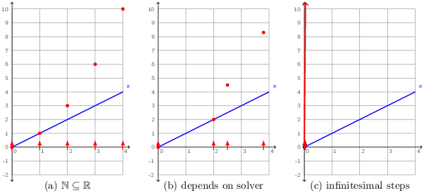
The signal x is continuous and o is discrete (due to the -> and pre operators). What can it mean to put them in parallel in this way? The meaning of x along is clear: ∀ t ∈ ℝ+, x(t) = t. It is shown in the three diagrams of figure 2.1 as a blue line that increases from zero with a constant slope. Each of the diagrams shows a different interpretation for o:

---

Figure 2.1: Possible interpretations of the wrong1 program.

---

We do not consider any of these three alternatives as acceptable. Instead, the compiler rejects wrong1 as invalid:

Similarly, a second program,

let hybrid wrong2() = o where
  rec der x = o init 0.0
  and o = 0.0 -> pre o +. 1.0

is also rejected as meaningless because o should be the discrete-time signal ∀ n ∈ ℕ, o(n) = n which cannot be integrated to produce x.

2.2.1  Typing Constraints.

The restrictions on mixing combinatorial, discrete-time, and continuous-time constructs are formalized as a typing system that statically accepts or rejects programs.

Every expression is associated to a kind k ∈ {A, D, C}. During typing, the compiler ensures that the following rules are satisfied:

1. The body of a combinatorial function (see section 1.1.4) must be of kind A. The body of a stateful function (declared as a node; see section 1.1.5) must be of kind D. Finally, the body of a continuous-time function (declared with the hybrid keyword) must be of kind C.
2. When the parallel composition of two (sets of) equations “E₁ and E₂” is expected to have kind k, then E₁ and E₂ must both also be of the same kind k. For instance, if E₁ and E₂ is expected to be combinatorial (k = A) then E₁ and E₂ must also both be combinatorial; if E₁ and E₂ is discrete (k = D) then both E₁ and E₂ must be discrete. Finally, if E₁ and E₂ is continuous (k = C) then both E₁ and E₂ must be continuous.
3. Any combinatorial equation or expression can be treated as either a discrete or a continuous one. In other words, A is a subkind of both D and C.

Thus, all sub-expressions in the body of a combinatorial function must be of kind A. All sub-expressions in the body of a node must be of kind A or of kind D. All sub-expressions in the body of a hybrid node must be of kind A or of kind C.

In addition to these basic rules, a computation with kind D can be placed in parallel with an expression of kind C provided it is sampled on a discrete clock. We adopt the following convention:

A clock is termed discrete if it has been declared so or if it is the result of a zero-crossing or a sub-sampling of a discrete clock. Otherwise, it is termed continuous.

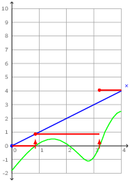
For example, the following function which composes an ODE and a discrete-time computation is correct. The value of x is added to that of o at every instant where tick is present. Between ticks, o is unchanged.

let hybrid correct(tick) = o where
  rec der x = 1.0 init 0.0
  and present tick -> do o = last o +. x done
  and init o = 0.0

The input tick has type zero, the type of zero-crossing events which are explained in the next section. The interpretation of this program is sketched in figure 2.2. The instants of activation of tick are generated (elsewhere) by monitoring a continuous expression. The value of o (in red) is recalculated at these instants by sampling the value at x and adding it onto the previous value, it is otherwise unchanged (that is, piecewise constant).

---

Figure 2.2: Interpretation of the (newly) correct program.

---

A formal presentation of the typing rules described in this section is available [2].

2.2.2  Zero-crossing Events

Zero-crossings are a standard mechanism used by numeric solvers to detect significant events. A solver recalculates the values of a set of zero-crossing expressions at each new approximation of the continuous state of a system. When one of the expressions changes sign between two successive approximations, the solver iterates to try to pinpoint the instant when the expression is equal to zero.

In Zélus, a zero-crossing expression is declared by the operator up(e). The language runtime detects when the value of the expression e changes from a negative value to a positive one during integration. The resulting events can be used to reset ODEs as illustrated in the following, classic example of a bouncing ball.

Consider a ball with initial position (x₀, y₀) and initial speed (x′₀, y′₀). Every time the ball hits the ground, it bounces but looses 20% of its speed. An example trajectory is depicted in figure 2.3.

---

Figure 2.3: The Bouncing Ball

---

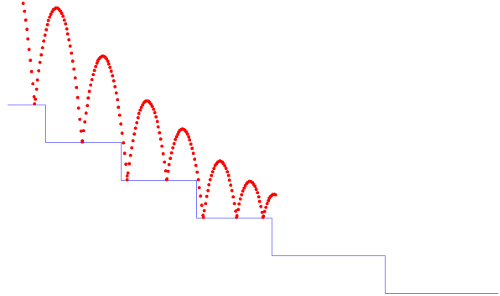
The source program is shown below. This version is slightly simplified compared to the version giving rise to figure 2.3: the steps are not modeled and we consider that the ground is at y=0. We will reconsider this detail when we reprogram the example in section 2.3.

let g = 9.81
let loose = 0.8

let hybrid bouncing(x0,y0,x'0,y'0) = (x,y) where
 rec der x = x' init x0
 and der x' = 0.0 init x'0
 and der y = y' init y0
 and der y' = -. g init y'0 reset up(-. y) -> -. loose *. last y'

The ODE defining y’ is reset every time -.y crosses zero. At this precise instant, the initial value of y’ is -. loose *. last y’. Exactly as in chapter 1, last y’ is the value of y’ at the previous instant. But the notion of previous instant for a continuous-time signal requires clarification. Mathematically, at the instant of a reset, we need to distinguish the value of y’ just before the reset and the new value that y’ takes at the instant of the reset. As y’ is a continuous-time signal, last y’ is the left limit of y’. It corresponds to the value of y’ computed during the integration process just preceding the discrete reaction that resets y’.

Replacing last y’ by y’ leads to an error of causality. Indeed, the current value of y’ would then depend instantaneously on itself. The compiler statically rejects such programs:

let hybrid bouncing(x0,y0,x'0,y'0) = (x,y) where
 rec der x = x' init x0
 and der x' = 0.0 init x'0
 and der y = y' init y0
 and der y' = -. g init y'0 reset up(-. y) -> -. loose *. y'

---

Figure 2.4: Trace of the sawtooth program.

---

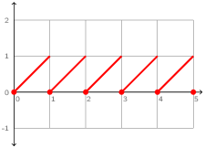
The sawtooth signal shown in figure 2.4 is another example of an ODE with reset. The signal x: ℝ⁺ ↦ ℝ⁺ is defined such that dx/dt(t) = 1 and x(t) = 0 if t∈ℕ, or as a hybrid node:

let hybrid sawtooth() = x where
  rec der x = 1.0 init 0.0 reset up(last x -. 1.0) -> 0.0

Each time last x -. 1.0 crosses zero from a negative to positive value, x is reset to zero. Note also the use of last to break what would otherwise be an invalid causality cycle.

2.2.3  Periodic Timers

A particular form of zero-crossings is provided to model timers. A timer with phase phase and period p generates an event at every instant where t = phase + n · period with n ∈ ℕ⁺. While such timers can be expressed directly using the features described in the previous two sections,

let hybrid timer(phase, p) = z where
  rec der t = 1.0 init -. phase reset z -> -. p
  and z = up(last t)

Zélus also provides a special period operator, which, for the moment at least, is restricted to timers of constant phase and period. For example, for a timer with phase = 10.3 and p = 20.5 one can write period 10.3(20.5). Such timers are not realized using zero-crossings, but rather by a dedicated and more efficient mechanism. At every discrete transition, the minimal ‘next value’ of all timers is computed to define the next integration horizon.

2.3  Hierarchical Automata and ODEs

We now illustrate how to combine ODEs with hierarchical automata using as an example, an hysteresis controller for a heater. We will first consider the heater dynamics. It has two modes: when active is true, the temperature increases; when active is false, it decreases. The hysteresis controller also has two modes. In the Idle mode, it outputs active = false until the temperature temp reaches the lower threshold t_min. The controller then stays in the Active mode until temp reaches the upper threshold t_max. The complete system is obtained by composing the heater and controller in parallel. Observe that the boolean signal active only changes when a zero-crossing occurs. This is a property guaranteed by the type system for all discrete (non-float) data types.

let c = 1.0
let k = 1.0
let temp0 = 0.0
let t_min = 0.0
let t_max = 1.0

(* an hysteresis controller for a heater: [c] and [k] are constant. *)
let hybrid heater(active) = temp where
  rec der temp = if active then c -. k *. temp else -. k *. temp init temp0

let hybrid hysteresis_controller(temp) = active where
  rec automaton
      | Idle -> do active = false until (up(t_min -. temp)) then Active
      | Active -> do active = true until (up(temp -. t_max)) then Idle

let hybrid main() = temp where
  rec active = hysteresis_controller(temp)
  and temp = heater(active)

The biggest difference between the automaton in the program above and those of previous programs is in the transition guards. The transition conditions of automata in a continuous context—that is, of kind C—may be either signal patterns, as described in section 1.4.11, or zero-crossing expressions, as in the example above. Notably, however, they may not be boolean expressions, though boolean expressions may still be combined with signal patterns. The equations within mode bodies inherit the kind of the automaton. In this example, we simply define active using constant expressions, but it would also have been possible to define signals by their derivatives (using der).

As always (continuous) automata may be nested hierarchically and composed in parallel. The extra structure is compiled away to generate a function that computes the temperature temp in tandem with a numeric solver and that monitors the active zero-crossing expression. The type system for automata [3] guarantees that mode changes will only occur at discrete instants, that is, in response to zero-crossing or timer events.

The ability to program with both automata and ODEs gives a restricted form of the hybrid automata of Maler, Manna, and Pnueli [15]. In particular, hybrid automata in Zélus are deterministic:

1. When several transitions can be fired, for example because several conditions are true, the first one in order is taken.
2. It is not possible to associate an invariant with a state. The current state is exited when a condition on an outgoing transition fires.

We will present a slightly more complicated hybrid automata by returning to the bouncing ball example of section 2.2.2. First we reprogram the vertical dynamics of the ball, this time using an external function, World.ground(), to retrieve the height of the ground as a function of the horizontal position.

(* [World.ground(x)] returns the position in [y] *)

let x_0 = 0.0
let y_0 = 8.0
let x_v = 0.72
let g = 9.81
let loose = 0.8

(* The bouncing ball *)
let atomic hybrid ball(x, y_0) = (y, y_v, z) where
  rec der y = y_v init y_0
  and der y_v = -. g init 0.0 reset z -> (-. loose *. last y_v)
  and z = up(World.ground(x) -. y)

We now incorporate these dynamics into an automaton with two modes. In Bouncing, it behaves as explained previously but for two details. When the velocity of the ball drops below a certain threshold, the system enters a Sliding mode and we gradually reduce the horizontal velocity. When Sliding, the ball only moves in the vertical dimension, until it reaches the edge of a step (as determined by a World.ground_abs() function).

let eps = 0.01

hybrid ball_with_modes(x_0, y_0) = (x, y) where
  rec init y_start = y_0
  and der x = x' init x_0
  and
  automaton
  | Bouncing ->
      (* the ball is falling with a possible bounce. *)
      local z, y_v in
      do
        (y, y_v, z) = ball(x, y_start)
      and x' = x_v until z on (y_v < eps) then Sliding(World.ground_abs(x),
                                                       World.ground(x))
  | Sliding(x0, y0) ->
      (* the ball is fixed, i.e., the derivative for y is 0 *)
      do
        y = y0
      and der x' = -0.8 *. x'
      until up(x -. x0) then do y_start = y in Bouncing
  end

This example demonstrates the hierarchical instantiation of hybrid nodes, the use of local variables in modes, shared variable resets on transition actions (...then do y_start = 0.0 in...) and a new on operator of type zero * bool -> zero which combines zero-crossing expressions and boolean conditions. The on operator emits an event when the zero-crossing occurs and the condition evaluates to true at that instant.

Futher examples are available online and in published papers [6].