Examples
Bouncing ball
A slight variation of the classic bouncing ball model: a ball bouncing down
a set of steps. The instants of impact are detected using zero crossings,
up(ground(x) -. y), which trigger a reset of the balls vertical velocity
to -0.8 its previous value.
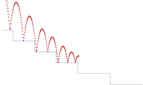
In the basic version of the program, the ball ‘falls through the floor’ due to limited floating-point precision.
 (** Bouncing ball. *)

(* [ground x] returns the position in [y] *)
let ground x = World.ground(x)
let ground_abs x = World.ground_abs(x)

let x_0 = 0.0
let y_0 = 8.0
let x_v = 0.72
let g = 9.81
let loose = 0.8

(* The bouncing ball *)
let hybrid ball(x, y_0) = (y, y_v, z) where
  rec
      der y = y_v init y_0
  and
      der y_v = -. g init 0.0 reset z -> (-. loose *. last y_v)
  and z = up(ground(x) -. y)

(* Main entry point *)
let hybrid main () =
  let der x = x_v init x_0 in
  let (y, _, z) = ball(x, y_0) in
  let ok = present (period (0.04)) -> () | z -> () in
  present ok() -> Showball.show (x fby x) (y fby y) x y;
  ()
With hybrid automata, it is instead possible to switch to a sliding dynamic when the balls vertical velocity becomes very small.
(** The same as the bouncing ball, this time with a mean *)
(* to avoid crossing the ground *)

(* [ground x] returns the position in [y] *)
let ground x = World.ground(x)
let ground_abs x = World.ground_abs(x)

let x_0 = 0.0
let y_0 = 10.0
let x_v = 0.45
let eps = 0.01

(* The bouncing ball with two modes. *)
hybrid ball(x_0, y_0) = (x, y, y_start) where
  rec init y_start = y_0
  and der x = x' init x_0
  and init x' = x_v
  and
  automaton
  | Bouncing ->
      (* the ball is falling with a possible bound. *)
      local z, y_v in
      do
        (y, y_v, z) = Ball.ball(x, y_start)
      until z on (y_v < eps) then Sliding(ground_abs x, ground(x))
  | Sliding(x0, y0) ->
      (* the ball slides, i.e., the derivative for y is 0 *)
      do
        y = y0
      and
          automaton
	  | Slide -> do der x' = -0.1 until up(-0.01 -. x') then Stop
	  | Stop -> do x' = 0.0 done
	  end
      until up(x -. x0) then do y_start = y in Bouncing
  end

(* Main entry point *)
let hybrid main () =
  let (x, y, y_start) = ball(x_0, y_0) in
  present (period (0.04)) -> Showball.show (x fby x) (y fby y) x y;
  ()
There is also a simpler model where the ball bounces up and down on the spot.
 (** Bouncing ball. *)

(* [ground x] returns the position in [y] *)
let ground x = Flatworld.ground(x)
let ground_abs x = Flatworld.ground_abs(x)

let x_0 = 5.0
let y_0 = 10.0
let g = 9.81
let loose = 0.8

(* The bouncing ball *)
let hybrid ball(x, y_0) = (y, y_v, z) where
  rec
      der y = y_v init y_0
  and
      der y_v = -. g init 0.0 reset z -> (-. loose *. last y_v)
  and z = up(ground(x) -. y)

(*
let hybrid gen(z) = (x0, v0) where
  rec init x0 = Random.float 4.0
  and init v0 = Random.float 4.0
  and present z ->
	do next x0 = Random.float 4.0 and v0 = Random.float 4.0 done
 *)

(* Main entry point *)
let hybrid main () =
  let rec (y, _, z) = ball(x_0, y_0)
  (* and (x_0, _) = gen(z) *) in
  present (period (0.04)) | z -> Showball.show x_0 (y fby y) x_0 y;
  ()
Bang-Bang Temperature Control
Requires: Lablgtk2
This model is a reimplementation of the Mathworks Simulink example Bang-Bang Control Using Temporal Logic. The main differences with the original model are:
We manually track the bias and slope for integers representing rational values.
We use int for the integer values rather than int8.
The top level of this example comprises three nodes:
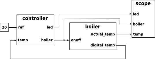
Controller
The controller is discrete. It takes two inputs:
reference temperature
This value is a constant 20°C, but it is encoded as a fixed-point integer so that it can be compared directly with the digital temperature value from the environment model. The reference temperature has a value between 0 (-15°C) and 255 (84.609375°C), i.e., a resolution of 0.390625 per bit (0.390625 = 5 / 256 / 0.05).
feedback temperature
A digital temperature measurement.
And provides two outputs:
led: the colour of a light emitting diode on the outside of the controller:
0=off,1=red(not heating),2=green(heating).
boiler: a signal that switches the boiler on (
1) or off (0).
The main part of the controller is an automaton with two top-level states:
Off: The boiler is off. The LED is flashed red at 0.1 Hz (5 secs off, 5 secs red).On: The boiler is on. The LED is flashed red at 0.5 Hz (1 sec off, 1 sec green).
The controller always remains in the Off state for at least 40 seconds,
after which it will switch to the On state if the temperature is less than
the reference temperature.
The controller may not remain in the On state for more than 20 seconds. It
will switch to the Off state if the temperature becomes greater than the
reference temperature.
The on state contains an internal automaton that stays in a High state from
t = 0 until the very first time that the measured temperature exceeds the
reference temperature (this is ensured by entry-by-history from Off). The
reason for this additional complication in the original Stateflow controller
is not clear; perhaps the intent was to heat at a faster rate the first time
the system is switched on? In our model, the effect is to delay an exit from
the On state by one reaction the first time the reference temperature is
attained.
Boiler
Boiler is a hybrid model of the boiler temperature and a digital thermometer.
The boiler temperature is modeled by a single integrator with an initial value of 15°C. This value (cools) at a rate of -0.1 / 25 when the boiler is off. It changes (heats) at a rate of 1.0 / 25 when the boiler is on.
The digital thermometer is modelled in some detail. Effectively, it takes a floating point temperature value in degrees centigrade and returns an integer between 0 and 255 representing that value (see the discussion above for the reference temperature).
The sensor itself has a bias of 0.75 and and a precision of 0.05, i.e., the
output voltage V is a function of the temperature T: V = 0.05 * T + 0.75. An
analog-to-digital converter (ADC) converts this voltage into an integer. By
scaling, quantization, and limiting.
Scope
Scope is a discrete node. It is triggered every sample_period to plot the
LED output, the boiler command, and the actual temperature against time.
Note that, even though all of these signals are continuous, they are plotted at discrete instants (as plotting is a side-effect) and the graph is thus (linearly) interpolated.
Simulation
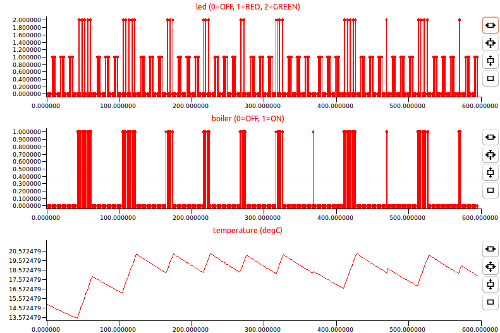
The simulation output shows a staircased increase in temperature from 15°C
at t = 0 to the 20°C just before t = 500. The initial rising edges have a
slope of 1.0/25 (the heating rate) and a duration of 20 seconds (the maximum
amount of time in the On state). The initial falling edges have a slope of
0.1/25 (the cooling rate) and a duration of 40 seconds (the minimum amount
of time in the Off state). After reaching the reference temperature, the
controller switches on and off to oscillate around the set-point.
The LED will flash green (2) during periods of heating, and red (1) during
periods of cooling, i.e., when not heating.
Note that the timing constants in the program have all been divided by 100
to speedup animation of the system. Another way to achieve the same effect
would have been to use the -speedup option available in compiled Zélus
programs.
(*
  Version of the Mathworks Simulink example:
      Bang-Bang Control Using Temporal Logic
 *)

(* time-scale factor *)
let tscale x = x *. 100.0

(* ** library functions ** *)
let hybrid integrator (i, u) = y where
  rec der y = tscale u init i

let discrete round x = floor (x +. 0.5)

(* ** model of analog-to-digital convertor ** *)

let discrete quantize (q, u) = q *. round(u /. q)

(* limiting without zero-crossings *)
let discrete limit (min, max, x) =
  if x >= max then max
  else if x <= min then min
  else x

let discrete adc (v) = pcm where
  rec vs = v *. (256.0 /. 5.0)
  and pcm = quantize (1.0, limit (0.0, 255.0, vs))

(* ** model of digital thermometer ** *)
let discrete digital_thermometer (temp) =
  let voltage = 0.05 *. temp +. 0.75 in
  let adv = adc (voltage) in
  int_of_float(adv)

(* signed fixed-point int from scale and bias *)
let discrete fixdt (s, b, v) = int_of_float ((v -. b) /. s)

(* ** model of boiler plant with an exponential ** *)
let hybrid boiler_exponential(k1, k2, is_on) = actual_temp where
  rec actual_temp = integrator (15.0, if is_on then k1 -. k2 *. actual_temp
                                      else -. k2 *. actual_temp)
  (* two modes. [is_on] is a boolean and will only change *)
  (* at a zero-crossing instant. *)

(* the one below is the Simulink version with an approximation by a *)
(* linear function *)
let hybrid boiler(is_on) =
  integrator (15.0, (if is_on then 1.0 else -0.1) /. 25.0)
    (* two modes. [is_on] is a boolean and will only change *)
    (* at a zero-crossing instant. *)

(* ** Bang-Bang Controller ** *)
let off   = 0
let red   = 1
let green = 2

let b_off  = false
let b_on   = true

let node wait (x) =
  let rec c = x -> pre (max 0 (c - 1)) in
  c = 0

let node at (x) =
  let rec c = 0 fby ((c + 1) mod x) in
  false -> (c = 0)

let node flash_led (color, delay) = led where
  automaton
  | Off -> do led = off   until (wait delay) then On
  | On  -> do led = color until (wait delay) then Off

let node controller (ref, temp) = (led, boiler) where
  rec cold = temp <= ref
  and automaton
  | Off ->
      do boiler = b_off
      and led = flash_led (red, 5)
      until (wait 40) & cold then On
  | On ->
      do boiler = b_on
      and led = flash_led (green, 1)
      until (not cold) then Off
      else  (at 20) then Off

(* ** main ** *)
let reference = fixdt (5.0 /. 256.0 /. 0.05, -. 0.75 /. 0.05, 20.0)

let hybrid model () = (led, on_off, actual_temp) where
  rec init led = red
  and init on_off = false
  and init digital_temp = 0
  and trigger = period (0.01)
  and present trigger ->
         do (led, on_off) = controller(reference, last digital_temp) done
  and present trigger ->
         do digital_temp = digital_thermometer (actual_temp) done
  and actual_temp = boiler(on_off)

open Scope (* Dump *)

let node bool_to_float(x) = if x then 1.0 else 0.0

let node plot (led, boiler, temp) =
  let s1 =
    scope (0.0, 2.0, ("led (0=OFF, 1=RED, 2=GREEN)", points true, float(led))) in
  let s2 =
    scope (0.0, 1.0, ("boiler (0=OFF, 1=ON)", points true, bool_to_float(boiler))) in
  let s3 =
    scope (11.0, 25.0, ("temperature (degC)", linear, temp)) in
  let rec t = 0.0 fby t +. 1.0 in
  window3 ("bangbang", 1600.0, t, s1, s2, s3)

let hybrid main () =
  let (led, on_off, actual_temp) = model () in
  let trigger = period (0.01) in
  present trigger -> plot (led, on_off, actual_temp) else ()
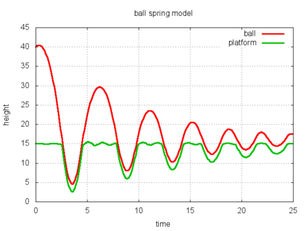
Ball and Spring
Author: Cyprien Lecourt

A ball bouncing on a spring with damping. This example is programmed as a two-state automaton. In the first state the ball and spring move separately: the ball decelerating and eventually falling back to the spring, and the spring oscillating with less and less energy. The second state is entered when the ball lands on the platform, in it the ball and platform move together until the ball becomes unstuck.
The calls to OCaml graphics for animating the system are written directly in a discrete node. Additional calls are added to log the system state to a file for graphing with gnuplot.
open Graphics
node start () =
  open_graph " 200x500";
  auto_synchronize false;
  set_line_width 4

(**Graphical features **)
(* [z]: ball height *)
(* [z_platform]: platform height *)
(* [rad]: ball radius *)
let discrete draw_ball_platform(z,z_platform,rad) =
  clear_graph ();
  let z = truncate (z *. 10.0) in
  let z_platform = truncate (z_platform *. 10.0) in
  set_color red;
  fill_circle 100 z (truncate(rad *. 10.0));
  set_color green;
  moveto 10 z_platform;
  lineto 190 z_platform;
  (* add spring zigzags *)
  let h = z_platform / 8 in
  moveto  20 z_platform;
  lineto 180 (z_platform - h);
  lineto  20 (z_platform - 2 ∗ h);
  lineto 180 (z_platform - 3 ∗ h);
  lineto  20 (z_platform - 4 ∗ h);
  lineto 180 (z_platform - 5 ∗ h);
  lineto  20 (z_platform - 6 ∗ h);
  lineto 180 (z_platform - 7 ∗ h);
  lineto  20 (z_platform - 8 ∗ h);
  lineto 180 (z_platform - 9 ∗ h);
  synchronize ()

(*physical constants for the ball*)
let g = 9.81
let m = 1.0
let radius = 2.0

(*and for the platform*)
let mp = 10.0
let k = 2.0
let f = 0.5 (* damping *)
let base_level = 15.0
let f_scratch = 0.1 (* level of interaction when stuck *)

open Dump

let hybrid simu (x_init) = x, xp where
  rec z = up(xp -. x)
  and rv = (2. *. mp *. last vp -. mp *. last v +. m *. last v) /. (mp +. m)
  and rvp = (2. *. m *. last v -. m *. last vp +. mp *. last vp) /. (mp +. m)
  and der v = -.g init 0.0 reset z -> rv
  and der vp = -. (k /. mp)  *. xp -. (f /. mp) *. vp init 0.0 reset z -> rvp
  and der x = v init x_init
  and der xp = vp init 0.0

  and der t = 1.0 init 0.0
  and _ = present (period (0.01)) | (init) ->
    let pos = scope2 (0.0, 100.0, ("ball", linear, x),
                      ("platform", linear, xp))
    in
    let w1 = window("ball_spring", 20.0, t, pos) in
    ()

let hybrid main () = () where
  rec init tmp = start ()
  and t = period (0.1)
  and x, xp = simu(10.)
  and z = x +. base_level
  and zp = xp +. base_level -. radius
  and _ = present t | (init) -> draw_ball_platform(z, zp, radius)
Self-Oscillating Adaptive System
Requires: Lablgtk2
This example comes from Chapter 10 of Åström and Wittenmark’s Adaptive Control (2nd edition).
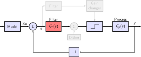
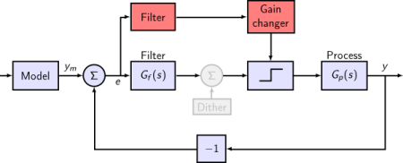
It involves the control of a simple process using adaptive relay feedback. Together, the process and relay incite limit cycle oscillations, giving systems with high feedback loop gain.
Three variations of the system are developed. The shared elements are incorporated into a single file:
(*
Example 10.2 (A basic SOAS)
from "Adaptive Control", 2e, Åström and Wittenmark, 2008
*)
(* ** library functions ** *)
(* linear first-order single-input single-output system *)
let hybrid siso_1o (a, b, c, d, u) = y where
rec der x1 = a *. x1 +. b *. u init 0.0
and y = c *. x1 +. d *. u
(* linear second-order single-input single-output system *)
let hybrid siso_2o ((a11, a12, a21, a22), (b1, b2), (c1, c2), d, u) = y where
rec der x1 = a11 *. x1 +. a12 *. x2 +. b1 *. u init 0.0
and der x2 = a21 *. x1 +. a22 *. x2 +. b2 *. u init 0.0
and y = c1 *. x1 +. c2 *. x2 +. d *. u
(* linear third-order single-input single-output system *)
let hybrid siso_3o ((a11, a12, a13, a21, a22, a23, a31, a32, a33),
(b1, b2, b3), (c1, c2, c3), d, u) = y where
rec der x1 = a11 *. x1 +. a12 *. x2 +. a13 *. x3 +. b1 *. u init 0.0
and der x2 = a21 *. x1 +. a22 *. x2 +. a23 *. x3 +. b2 *. u init 0.0
and der x3 = a31 *. x1 +. a32 *. x2 +. a33 *. x3 +. b3 *. u init 0.0
and y = c1 *. x1 +. c2 *. x2 +. c3 *. x3 +. d *. u
(* ideal relay model *)
let hybrid relay (d, e) = u where
u = present up(e) | up(-. e) | (disc(e)) | (init)
-> if e >= 0.0 then d else -. d init 0.0
(* ** model ** *)
(* feed-forward reference model
damping factor z = 0.7;
natural frequency w = 1.0 rad/sec;
The state-space realization can be calculated in Matlab:
[A, B, C, D] = ord2(1.0, 0.7)
Or in Scilab:
s = %s; wn = 1.0; zeta = 0.7;
tf2ss(syslin('c', wn^2, s^2 + 2*zeta*wn*s + wn^2))
*)
let hybrid reference u =
siso_2o ((0.0, 1.0, -1.0, -1.4), (0.0, 1.0), (1.0, 0.0), 0.0, u)
let hybrid command () = u where
automaton
| S0 -> do u = 1.0 until (period (17.5 | 17.5)) then S1
| S1 -> do u = -1.0 until (period (35.0 | 35.0)) then S2
| S2 -> do u = 1.0 done
(* compensation network
s + 5
G_f(s) = 1.2 * ( -------- )
s + 15
The state-space realization can be calculated in Matlab:
[a, b, c, d] = ss(1.2 * tf([1 5], [1 15]))
or in Scilab:
s = poly(0, 's')
[a, b, c, d] = abcd(tf2ss(1.2 * (s + 5) / (s + 15)))
*)
let hybrid g_f u = siso_1o (-15.0, 4.0, -3.0, 1.2, u)
(* up-logic gain changer *)
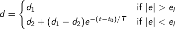
(* The initial state should be D1 when |e| > e_l *)
let hybrid gain_changer (d1, d2, e_l, e) = d where
automaton
| D2 -> local t in
do
der t = 1.0 init 0.0
and d = d2 +. (d1 -. d2) *. exp(-.t)
until up(abs_float e -. e_l) then D1
| D1 -> do d = d1 until up(e_l -. abs_float e) then D2
(* The process:
G(s) = K * alpha
-------------------
s(s + 1)(s + alpha)
"The nominal values of the parameters are K = 3, ..., and alpha = 20."
The state-space realization can be calculated in Matlab:
sys1 = tf(60, [1 21 20 0])
[a, b, c, d] = ss(sys1)
"The process gain is suddenly increased by a factor of 5 at t = 25."
sys2 = 5 * sys1
[a, b, c, d] = ss(sys2)
And similarly in Scilab:
s=%s
sys1 = 60 / (s * (s + 1) * (s + 20))
[a, b, c, d] = abcd(sys1)
sys2 = 5 * sys1
[a, b, c, d] = abcd(sys2)
*)
let hybrid process u = y where
rec automaton
| G5 -> do b1 = 4.0 and c3 = 3.750 until (period (25.0 | 25.0)) then G15
| G15 -> do b1 = 8.0 and c3 = 9.375 done
and y = siso_3o ((-21.0, -5.0, 0.0,
4.0, 0.0, 0.0,
0.0, 1.0, 0.0),
(b1, 0.0, 0.0), (0.0, 0.0, c3), 0.0, u)
open Scope (* Dump *)
let hybrid plot (title, y, y_m, u, e) = () where
_ = present (period (0.08)) -> (
let
rec s1 = scope2 (-1.5, 1.5, ("y_m", linear, y_m),
("y", linear, y))
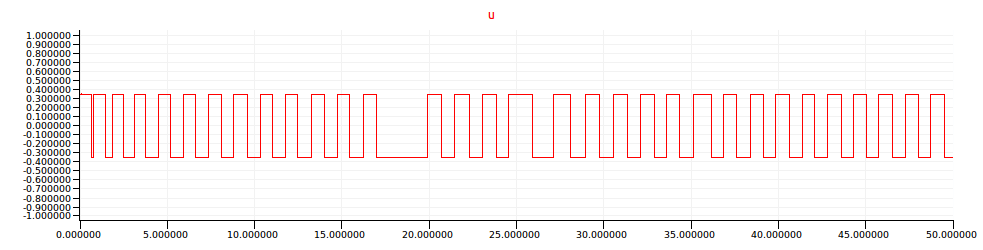
and s2 = scope (-1.0, 1.0, ("u", square, u))
and s3 = scope (-1.0, 1.3, ("e", linear, e))
and t = 0.0 fby t +. 0.08
in window3 (title, 50.0, t, s1, s2, s3))
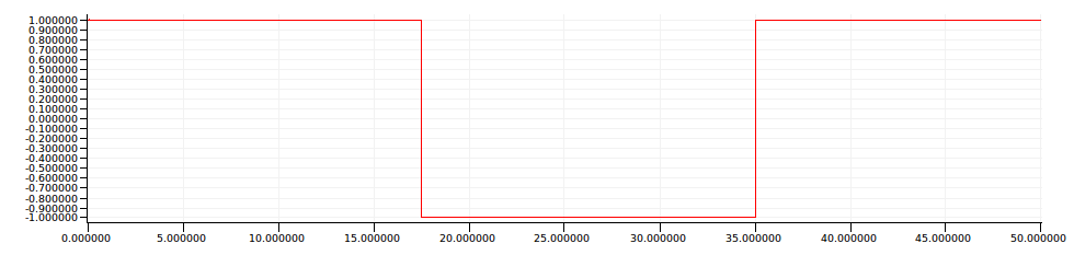
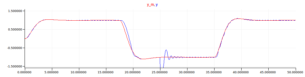
The models are tested over a period of 50s in response to a command
signal which starts at 1 initially, drops to 0 at 17.5 seconds, and
then rises to 1 again at 35 seconds.
The command signal is defined using a hybrid automaton in a node called
command.
The process to be controlled is described by the transfer function:
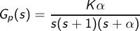
where, initially, K = 3 and α = 20, but where the process gain is suddenly increased by a factor of 5 at t = 25. The state-space realizations of these two systems are readily calculated in either Matlab:
sys1 = tf(60, [1 21 20 0])
[a, b, c, d] = ss()

sys2 = 5 * sys1
[a, b, c, d] = ss(sys2)
or Scilab:
s=%s
sys1 = 60 / (s * (s + 1) * (s + 20))
[a, b, c, d] = abcd(sys1)

sys2 = 5 * sys1
[a, b, c, d] = abcd(sys2)
We implement them in a node called process using a hybrid automaton and a
generic siso_3o node that takes the state-space matrices as tupled
arguments.
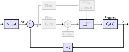
Basic SOAS
The first model comprises a simple feedback loop—relay, process, and inverter—that tries to follow the reponse of a reference model to the command signal. Other elements will be added successively.
(*
    Example 10.2 (A basic SOAS)
    from "Adaptive Control", 2e, Åström and Wittenmark, 2008
 *)

open Soas

let hybrid main () = () where
  rec i = command ()
  and y_m = reference i
  and u = relay (0.35, e)
  and e =  y_m -. y

  (* Rmk: we should be able to put the automaton below *)
  (* into a function. We can not for the moment as there *)
  (* is no inlining of function call a priori *)
  and automaton
      | G3  -> do b1 = 4.0 and c3 = 3.750 until (period (25.0 | 25.0)) then G15
      | G15 -> do b1 = 8.0 and c3 = 9.375 done

  and der x1 = -21.0 *. x1  +.  -5.0 *. x2  +.  b1 *. u init 0.0
  and der x2 =   4.0 *. x1 init 0.0
  and der x3 =   1.0 *. x2 init 0.0
  and y = c3 *. x3

  and () = plot ("Basic SOAS", y, y_m, u, e)
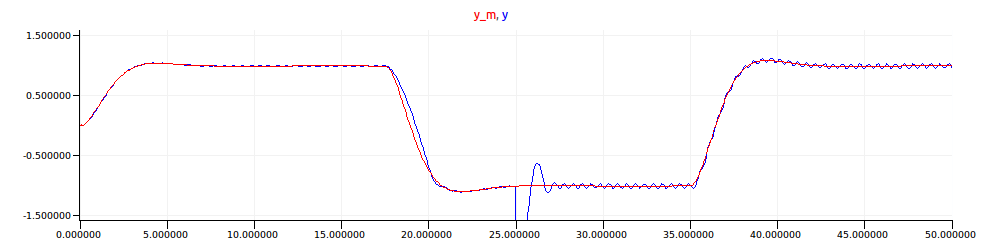
The reference model is described as a second order system with damping coefficient ζ = 0.7 and natural frequency ω_n = 1 rad/sec. Its state-space realization is readily calculated in either Matlab:
[A, B, C, D] = ord2(1.0, 0.7)
or Scilab:
s = %s; wn = 1.0; zeta = 0.7;
tf2ss(syslin('c', wn^2, s^2 + 2*zeta*wn*s + wn^2))
We express it in a node called reference using a generic siso_2o node.
The response of the reference model to the command input is shown in red below. The actual output of the feedback loop is shown in blue.
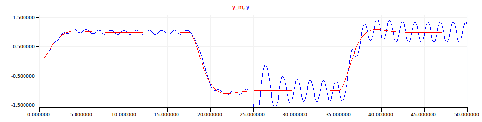
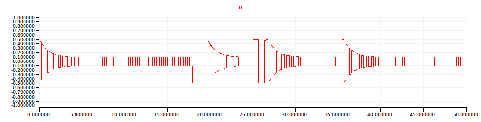
The relay is modelled in a node called relay using a hybrid
automaton that alternates between High (output = d) and Low (output =
-d) states in response to zero-crossings on its input signal.
The relay’s value is shown below.
SOAS with lead network
The next model augments the basic model with a compensation network that adds a phase lead of -π.
(*
    Example 10.2 (A basic SOAS)
    from "Adaptive Control", 2e, Åström and Wittenmark, 2008
 *)

open Soas

let hybrid main () = () where
  rec i = command ()
  and y_m = reference i
  and u = relay (0.35, g_f e)
  and e =  y_m -. y

  (* Rmk: we should be able to put the automaton below *)
  (* into a function. We can not for the moment as there *)
  (* is no inlining of function call a priori *)
  and automaton
      | G3  -> do b1 = 4.0 and c3 = 3.750 until (period (25.0 | 25.0)) then G15
      | G15 -> do b1 = 8.0 and c3 = 9.375 done

  and der x1 = -21.0 *. x1  +.  -5.0 *. x2  +.  b1 *. u init 0.0
  and der x2 =   4.0 *. x1 init 0.0
  and der x3 =   1.0 *. x2 init 0.0
  and y = c3 *. x3

  and () = plot ("SOAS with lead network", y, y_m, u, e)
The compensation filter is defined as a transfer function:
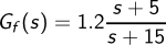
which is implemented in the node g_f using the generic node siso_1o
after having calculated its state-space realization in either
Matlab:
[a, b, c, d] = ss(1.2 * tf([1 5], [1 15]))
or Scilab:
s = poly(0, 's')
[a, b, c, d] = abcd(tf2ss(1.2 * (s + 5) / (s + 15)))
The compensation filter decreases the amplitude of oscillation while maintaining the reponse speed, as can be seen in the simulation results below.
SOAS with lead network and gain changer
A gain changer is added in the final model. It uses so called up logic to speed up the controller’s reponse.
(*
    Example 10.2 (A basic SOAS)
    from "Adaptive Control", 2e, Åström and Wittenmark, 2008
 *)

open Soas

let hybrid main () = () where
  rec i = command ()
  and y_m = reference i
  and u = relay (gain_changer (0.5, 0.1, 0.1, e), g_f e)
  and e =  y_m -. y

  (* Rmk: we should be able to put the automaton below *)
  (* into a function. We can not for the moment as there *)
  (* is no inlining of function call a priori *)
  and automaton
      | G3  -> do b1 = 4.0 and c3 = 3.750 until (period (25.0 | 25.0)) then G15
      | G15 -> do b1 = 8.0 and c3 = 9.375 done

  and der x1 = -21.0 *. x1  +.  -5.0 *. x2  +.  b1 *. u init 0.0
  and der x2 =   4.0 *. x1 init 0.0
  and der x3 =   1.0 *. x2 init 0.0
  and y = c3 *. x3

  and () = plot ("SOAS with lead network and gain changer", y, y_m, u, e)
A gain changer increases the relay’s amplitude (d) when a specified
tolerance (e_l) is exceeded.
This logic is readily implemented in the gain_changer node using a hybrid
automaton.
The simulation results show that the new controller responds with smaller amplitude oscillations to the system with higher gain, without losing performance for the system with smaller gain.
The effect of the gain changing logic on the relay output is evident in the exponential envelopes on the signal shown below.
Sticky Masses
Requires: Lablgtk2 (glMLite)
This example is based on example 6.8 in Edward A. Lee and Pravin Varaiya, Structure and Interpretation of Signals and Systems, Second Edition, and the Ptolemy II model by Jie Liu, Haiyang Zheng, and Edward A. Lee.
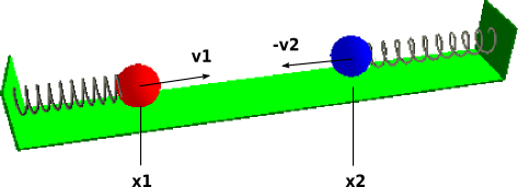
The model comprises two sticky round masses, each on the end of a spring. The other ends of the springs are tied to opposing walls. After the springs are compressed (or extended) and released the masses oscillate back and forth, and may collide. After a collision, the masses remain stuck together until the pulling forces from the springs are greater than a stickiness value (which decreases exponentially after a collision).
(* ** Parameters ** *)

(* neutral positions of the two masses *)
let p1 = 1.25
let p2 = 1.75

(* initial positions of the two masses: y1_i < y2_i *)
let x1_i = 0.0
let x2_i = 3.0

(* spring constants *)
(* let k1 = 4.0 (* exhibits problem *) *)
let k1 = 1.0
let k2 = 2.5 (* 2.0 *)

(* masses *)
let m1 = 1.5
let m2 = 1.0

(* stickyness *)
let stickiness_max = 10.0
let tau = 0.5

(* ** Model ** *)

let hybrid sticky () =
  ((x1, v1), (x2, v2), pull, stickiness_out, total) where
  rec der x1 = v1 init x1_i
  and der x2 = v2 init x2_i
  and init v1 = 0.0
  and init v2 = 0.0
  and total = 0.5 *. m1 *. v1 *. v1 +. 0.5 *. m2 *. v2 *. v2 +.
              0.5 *. k1 *. (x1 -. p1) *. (x1 -. p1) +.
              0.5 *. k2 *. (x2 -. p2) *. (x2 -. p2)
  and automaton
      | Apart ->
          local mediant in
          do  der v1 = k1 *. (p1 -. x1) /. m1
          and der v2 = k2 *. (p2 -. x2) /. m2
          and mediant = (v1 *. m1 +. v2 *. m2) /. (m1 +. m2)
          and pull = 0.0
          and stickiness_out = 0.0
          until up (x1 -. x2) then
             do next v1 = mediant
             and next v2 = mediant in Together
      | Together ->
          local y_dot_dot, stickiness in
          do  pull =
               abs_float (-. last x1 *. (k1 +. k2) +. (k2 *. p2 -. k1 *. p1))
          and y_dot_dot =
               (k1 *. p1 +. k2  *. p2 -. (k1 +. k2) *. last x1) /. (m1 +. m2)
          and der v1 = y_dot_dot
          and der v2 = y_dot_dot
          and der stickiness = -. stickiness /. tau init stickiness_max
          and stickiness_out = stickiness
          until (init) on (pull >= stickiness) then Apart
           else up (pull -. stickiness) then Apart

(* ** plotting ** *)

open Scope

let node plot (t, (y1, y1_dot), (y2, y2_dot), pull_force, stickiness, total) =
  let s1 = scope2 (0.0, 3.0, ("p1", linear, y1), ("p2", linear, y2)) in
  let s2 = scope2 (-1.5, 1.5, ("v1", linear, y1_dot), ("v2", linear, y2_dot)) in
  let s3 = scope2 (0.0, stickiness_max, ("Pulling force", linear, pull_force),
                                        ("Stickiness", linear, stickiness)) in
  let s4 = scope (0.0, 3.0, ("Total Energy", linear, total)) in
  window4 ("sticky springs", 30.0, t, s1, s2, s3, s4)

(* ** main ** *)

let hybrid main () =
  let der t = 1.0 init 0.0 in
  let ((y1, y1_dot), (y2, y2_dot), pull_force, stickiness, total) = sticky () in
  present
     (period (0.10)) ->
       plot (t, (y1, y1_dot), (y2, y2_dot), pull_force, stickiness, total);
  ()
Backhoe
Requires: Lablgtk2
The Backhoe loader is an original example that we developed to teach reactive programming.
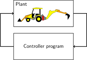
The model comprises two interconnected elements:
- a continuous model of the plant (parts of the backhoe)
- a discrete controller
The original programming challenge focused on the discrete controller, but expressing the continuous dynamics is also an interesting programming problem, as is interfacing the two models.
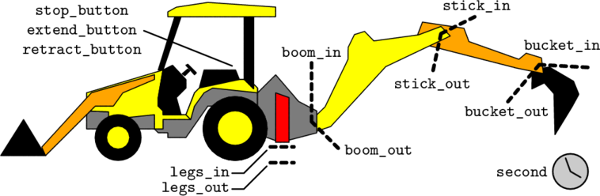
The discrete controller receives input from sensors which are defined inside
the continuous model. There are sensors for each of three buttons
(stop_button, extend_button, and retract_button), for indicating
whether the legs are fully retracted (legs_in) or fully extended
(legs_out), and for indicating whether each of the rear segments is fully
retracted (*_in) or fully extended (*_out).

There are control signals for three lamps (alarm_lamp, done_lamp, and
cancel_lamp) and for triggering leg extension (legs_extend), leg
retraction (legs_retract), and stopping leg motion (legs_step). There
are three control signals pel segment: setting an internal valve for pushing
(*_push), or for pulling (*_pull), and for driving hydraulic fluid
through the valve (*_drive). It is assumed that a lower-level controller
maintains a segments position when it is not being driven.
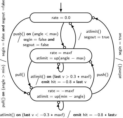
Each segment is modelled using set of equations that include a hybrid automaton. Two types of dynamics are modelled: moving and stopping with momentum (modelled as a Proportional-Integral controller) and bouncing at the limits of movement (modelled as instantaneous reset).
let node aftern (n, t) = (c = n) where
  rec c = 0 fby min (if t then c + 1 else c) n

let node blink (n, t) = x where
  automaton
  | On  -> do x = true  until (aftern (n, t)) then Off
  | Off -> do x = false until (aftern (n, t)) then On

let node blink2(ton, toff, t) = x where
  automaton
  | On  -> do x = true  until (aftern (ton, t)) then Off
  | Off -> do x = false until (aftern (toff, t)) then On

let node leg_controller
    ((legs_in, legs_out), (stop_button, retract_button, extend_button), second) =
    ((legs_extend, legs_retract, legs_stop), alarm, extended)
  where
  rec init alarm = false
  and init extended = false
  and automaton
      | LegsIn ->
          do alarm = false
          until extend_button then LegsMoving(true)

      | LegsMoving(extend) -> do
          automaton
             | Initial ->
                 do
                 until extend       then Extending
                  else (not extend) then Retracting

             | Extending ->
                 do
                   emit legs_extend
                 until stop_button    then Stopped
                  else retract_button then Retracting

             | Retracting ->
                 do
                   emit legs_retract
                 until stop_button   then Stopped
                  else extend_button then Extending

             | Stopped ->
                 do
                   emit legs_stop
                 until extend_button  then Extending
                  else retract_button then Retracting

             and alarm = false -> not (pre alarm)
             and extended = false

          until legs_extend(_)  & legs_out then LegsOut
           else legs_retract(_) & legs_in  then LegsIn
           else (aftern(20, second))       then Error

      | LegsOut ->
          do
            extended = true and alarm = false
          until retract_button then LegsMoving(false)

      | Error ->
          do
                alarm = true
            and emit legs_retract
          until legs_in then LegsIn

let node sampled_controller
  ((leg_sensors, (boom_in, boom_out), (stick_in, stick_out), (bucket_in, bucket_out)),
   (stop_button, retract_button, extend_button), second)
  =  ((boom_push,   boom_pull,   boom_drive),
      (stick_push,  stick_pull,  stick_drive),
      (bucket_push, bucket_pull, bucket_drive),
      (legs_extend, legs_retract, legs_stop),
      (alarm_lamp, done_lamp, cancel_lamp))
  where
  rec init boom_drive   = false
  and init stick_drive  = false
  and init bucket_drive = false

  and init alarm_lamp  = false
  and init done_lamp   = false
  and init cancel_lamp = false

  and init legs_extended = false

  and automaton
      | Legs ->
          do alarm_lamp  = leg_alarm
          and done_lamp   = false
          and ((legs_extend, legs_retract, legs_stop), leg_alarm, legs_extended)
                  = leg_controller (leg_sensors, (stop_button, retract_button, extend_button), second)
          until (legs_extended) then Stable

      | Stable ->
          do alarm_lamp  = false
          and done_lamp   = true
          and cancel_lamp = false
          until extend_button  then Dig
           else retract_button continue Legs

      | Dig ->
          local finished in
          do init finished = false
          and
          automaton
            | Move ->
                do done_lamp = false
                and alarm_lamp = blink(2, second)
                and automaton
                  | RaiseStickBucket ->
                      do emit stick_pull  and stick_drive = true
                      and emit bucket_pull and bucket_drive = true
                      unless (stick_in && bucket_in) then LowerBoom

                  | LowerBoom ->
                      do emit boom_push and boom_drive = true
                      and bucket_drive = false and stick_drive = false
                      unless boom_out then FillStickBucket

                  | FillStickBucket ->
                      do emit stick_push  and stick_drive = true
                      and emit bucket_push and bucket_drive = true
                      and boom_drive = false
                      unless (stick_out && boom_out) then RaiseBoom

                  | RaiseBoom ->
                      do emit boom_pull and boom_drive = true
                      and bucket_drive = false and stick_drive = false
                      unless (boom_in) then Finished

                  | Finished ->
                      do finished = true done

                until (stop_button) then Pause

            | Pause ->
                do alarm_lamp = false
                and done_lamp  = blink2(4, 2, second)
                and boom_drive = false
                and stick_drive = false
                and bucket_drive = false
                until (extend_button) continue Move
                 else (retract_button || aftern(30, second)) then Cancel

            | Cancel ->
                do cancel_lamp = blink(1, second)
                and alarm_lamp = false
                and done_lamp  = false

                and emit boom_pull   and boom_drive   = true
                and emit stick_push  and stick_drive  = true
                and emit bucket_push and bucket_drive = true

                and finished = boom_in && stick_out && bucket_out
                done

            until (finished) then Stable

let hybrid main () = () where
  rec init sensors = ((false, false), (false, false),
                      (false, false), (false, false))

  and init boom_drive = false
  and init stick_drive = false
  and init bucket_drive = false
  and init alarm_lamp = false
  and init done_lamp = false
  and init cancel_lamp = false

  and present sample ->
        do ((boom_push, boom_pull, boom_drive),
           (stick_push, stick_pull, stick_drive),
           (bucket_push, bucket_pull, bucket_drive),
           (legs_extend, legs_retract, legs_stop),
           (alarm_lamp, done_lamp, cancel_lamp)) =
                          sampled_controller (last sensors, Backhoedyn.buttons (), second)
        done

  and sensors =
        Backhoedyn.model ((boom_push, boom_pull, boom_drive),
                          (stick_push, stick_pull, stick_drive),
                          (bucket_push, bucket_pull, bucket_drive),
                          (legs_extend, legs_retract, legs_stop),
                          (alarm_lamp, done_lamp, cancel_lamp))

  and sample = period (0.2)

  (* and second = present sample -> not (last second) init true *)
  (* and second = present (init) | sample -> true fby not (second) init true *)

  and second = present sample -> true -> not (last second) init true
(** Model constants *)

let boom_rate   =  1.6
let stick_rate  = 10.0
let bucket_rate =  2.8
let leg_rate    = 32.0

(** Model components *)

let hybrid segment ((min, max, i), maxf, (push, pull, go))
 = ((segin, segout), angle) where

 rec der angle = v init i
 and error = v_r -. v
 and der v = (0.8 /. maxf) *. error +. 0.2 *. z init 0.0
             reset hit(v0) -> v0
 and der z = error init 0.0 reset hit(_) -> 0.0
 and v_r = if go then rate else 0.0
 and init segin = angle <= min
 and init segout = angle >= max

 and automaton
   | Stuck -> do
        rate = 0.0
      until push() on (angle < max) then
        do segin = false and segout = false in Pushing
      else  pull() on (angle > min) then
        do segin = false and segout = false in Pulling

   | Pushing -> local atlimit in
      do
        rate = maxf
        and atlimit = up(angle -. max)
      until atlimit on (last v > 0.1 *. maxf) then do
               emit hit = -0.3 *. last v in Pushing
      else (atlimit) then do segout = true and emit hit = 0.0 in Stuck
      else pull() then Pulling

   | Pulling -> local atlimit in
      do
        rate = -. maxf
        and atlimit = up(min -. angle)
      until atlimit on (last v < -0.1 *. maxf) then do
               emit hit = -0.3 *. last v in Pulling
      else  (atlimit) then do segin = true and emit hit = 0.0 in Stuck
      else  push() then Pushing

let hybrid legsegment ((min, max, i), rate, (extend, retract, stop)) =
  ((segin, segout), pos) where

  rec init pos = i
  and init segin  = pos <= min
  and init segout = pos >= max

  and automaton
    | Stationary ->
        do
          der pos = 0.0
        until extend() on (not segout)
          then do next segin = false in Extending
        else  retract() on (not segin)
          then do next segout = false in Retracting

    | Extending ->
        do
          der pos = rate
        until up(pos -. max)
          then do next segout = true in Stationary
        else  stop()         then Stationary
        else  retract()      then Retracting

    | Retracting ->
        do
          der pos = -. rate
        until up(min -. pos) then do next segin = true in Stationary
        else  stop()         then Stationary
        else  extend()       then Extending


(** Put the model together and link it to the GUI *)

open Backhoegui

let node buttons () = showsample ()

let hybrid model
  (boom_control, stick_control, bucket_control, leg_control, lamp_control) =

  let (boom_sensors, boom_ang)
      = segment (boom_range, boom_rate, boom_control)

  and (stick_sensors, stick_ang)
      = segment (stick_range, stick_rate, stick_control)

  and (bucket_sensors, bucket_ang)
      = segment (bucket_range, bucket_rate, bucket_control)

  and (leg_sensors, leg_pos)
      = legsegment (leg_range, leg_rate, leg_control)

  and refresh_rate = period (0.1) in

  let
  rec (alarm_lamp, done_lamp, cancel_lamp) = lamp_control
  and _ =
    present
    | refresh_rate ->
          showupdate (leg_pos, boom_ang, stick_ang, bucket_ang,
                               alarm_lamp, done_lamp, cancel_lamp)
  in
  (leg_sensors, boom_sensors, stick_sensors, bucket_sensors)
Further details can be found in the paper Zélus: A Synchronous Language with ODEs.
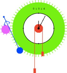
Pendulum Clock
Author: Guillaume Baudart
This model was made to celebrate Albert Benveniste’s 65th birthday in honour of “The old fashioned Signal watch”.
The clock features an escapement that regulates the movement of two cogs
according to the oscillations of a pendulum. The escapement node generates
four events as the pendlum moves: tic and toc as the smaller, pink cog
is caught by the escapement and stopped from moving, and rtic and rtoc
as it is released and allowed to turn. When the ping cog is free, then
bigger, green cog can turn pulled by the falling atwood masses.
This in turn moves the clock hands.
The clockwatch node is an automaton with four modes:
Move: the cogs are free to turn.Stop: the cogs are trapped by the escapement.Exhausted: there is no energy left in the masses.Setting: energy is added to the mass system.
A sound is emitted whenever the escapement catches (on tic and toc). The
spacebar is used to reset the position of the masses. The system state is
drawn by an external (OCaml) function called draw_system.
open Draw

(******************* Pendulum Clock **********************)

let g = 9.81
let pi = 3.1415

(* Pendulum parameters *)
let l = 1.5
let theta0 = 0.5

(* Atwood parameters *)
let m1 = 11.
let m2 = 10.
let h0 = 2.

(* escapement parameters *)
let thetac = 0.4

let hybrid pendulum theta0 = theta where
  rec der thetap =  -. (g /. l) *. sin (theta) init 0.0
  and der theta = thetap init theta0

let hybrid atwood h0 = (h,v) where
  rec der v = g *. (m2 -. m1) /. (m2 +. m1) init 0.0
  and der h = v init h0

let hybrid hand (ti, v) = t where
  rec der t = -. v init ti

let hybrid set hi = h where
  rec der h' = 0.5 init hi
  and h = min h0 h'

let hybrid escapement theta = (tic, rtic, toc, rtoc) where
  rec present
        | up (-. theta -. thetac) -> do emit tic = () done
        | up (theta +. thetac) -> do emit rtic = () done
        | up (theta -. thetac) -> do emit toc = () done
        | up (-. theta +. thetac) -> do emit rtoc = () done

let hybrid clockwatch (h0, t0, theta, r) = (h, t, active) where
  rec (tic, rtic, toc, rtoc) = escapement theta
  and init active = true
  and init t = t0
  and init h = h0
  and automaton
      | Move(hi, ti) ->
          do (h,v) = atwood hi
          and t = hand (ti,v)
          until tic() | toc() then Stop(h,t)
          else up (-. h) then Exhausted(t)
          else r() then Setting(h,t)
      | Stop(hi, ti) ->
          do active = true
          until rtic() | rtoc() then Move(hi,ti)
          else r() then Setting (h,t)
      | Exhausted(ti) ->
          do active = false
          until r() then Setting(h,ti)
      | Setting (hi, ti) ->
          do h = set hi
          and active = false
          until r() then Stop (h,t)
  init Move(h0, t0)


let node digitalwatch (hi,mi,si) = (h,m,s) where
  rec s = si fby (s+1) mod 60
  and m = mi -> (if ((s = 0) && (s <> 0 fby s)) then (pre m) + 1 else pre m) mod 60
  and h = hi -> (if ((m = 0) && (m <> 0 fby m)) then (pre h) + 1 else pre h) mod 24


(********** Simulation ************)

let hybrid keyboard () = go where
  rec init ok = false
  and s = period (0.04)
  and present s -> do ok = input () done
  and present s on ok -> do emit go = () done

let hybrid sampled_digitalwatch (tic, toc, active, hi,mi,si) = (h,m,s) where
  rec init s = si
  and init m = mi
  and init h = hi
  and present tic() on active | toc() on active ->
      (* do h,m,s = digitalwatch (h,m,s) done *)
      local h',m',s' in
      do
        h', m', s' = digitalwatch (h,m,s)
        and next h = h'
        and next m = m'
        and next s = s'
      done

let hybrid main () =
  let ok = period (0.04) in
  let theta = pendulum theta0 in
  let (tic, _, toc, _) = escapement theta in
  let r = keyboard () in
  let (h, t, active) = clockwatch (h0, 0.0, theta,r) in
  let thb = t *. (24. /. 30.) in
  let thl = thb /. 60. in

  let twb = t /. 3. in
  let twl = -.t *. (120. /. 20.) /. 3.  in

  let (hh,mm,ss) = sampled_digitalwatch(tic, toc, active, 0, 0, 1) in

  present ok -> draw_system (l, thetac, theta, h0, h, thb, thl, twb, twl, hh, mm, ss)
        | tic() on active -> play_tic ()
        | toc() on active  -> play_toc ();
    ()
Spring-driven Watch
Author: Guillaume Baudart
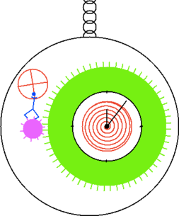
This model was made to celebrate Albert Benveniste’s 65th birthday in honour of “The old fashioned Signal watch”.
The watch features an escapement that regulates the movement of two cogs
according to the back and forth rocking of a regulator wheel. The
escapement node generates four events as the regulator moves: tic and
toc as the smaller, pink cog is caught by the escapement and stopped from
moving, and rtic and rtoc as it is released and allowed to turn. When
the ping cog is free, then bigger, green cog is pushed by the balance
spring. This in turn moves the clock hands. The clockwatch node is an
automaton with four modes:
Move: the cogs are free to turn.Stop: the cogs are trapped by the escapement.Exhausted: there is no energy left in the masses.Setting: energy is added to the mass system.
A sound is emitted whenever the escapement catches (on tic and
toc). As an added bonus, the entire system can be made to swing back
and forth. The watch then behaves as a pendulum controlled by an
automaton with two modes.
Stop: The pendulum does not move.Move: The pendulum starts moving with a fixed initial angular speed.
The user can switch between the two behaviors by pressing the m key.
The system state is drawn by an external (OCaml) function called
draw_system.
open Draw

(******************* Pendulum Clock **********************)


let x0 = 400.
let y0 = 600.


let g = 9.81
let l = 4.

let k1 = 5.
let k2 = 1.
let pi = 3.1415

(* Pendulum parameters *)
let theta0 = 1.

(* Spring parameters *)
let h0 = 2.

(* escapement parameters *)
let thetac = 0.4

let hybrid pendulum (theta0, thetap0) = theta where
   rec der thetap =  -. (g /. (10. *. l)) *. sin (theta) init thetap0
   and der theta = thetap init theta0

let hybrid chain (theta0, thetap0, move) = theta where
  rec automaton
      | Stop(th) ->
          do theta = th
          until move() then Move(theta)
      | Move(th) ->
          do theta = pendulum(th, thetap0)
          until move() then Stop(theta)
  init Stop(0.0)

let hybrid balance theta0 = theta where
  rec der thetap =  -. k1 *. theta init 0.0
  and der theta = thetap init theta0

let hybrid spring h0 = h where
  rec der v = -. k2 *. h init 0.0
  and der h = v init h0

let hybrid hand ti = t where
  rec der t' = 1.0 init 0.0
  and der t = t' init ti

let hybrid set hi = h where
  rec der h' = 0.5 init hi
  and h = min h0 h'

let hybrid escapement theta = (tic, rtic, toc, rtoc) where
  rec present
        | up (-. theta -. thetac) -> do emit tic = () done
        | up (theta +. thetac) -> do emit rtic = () done
        | up (theta -. thetac) -> do emit toc = () done
        | up (-. theta +. thetac) -> do emit rtoc = () done

let hybrid clockwatch (h0, t0, theta, r) = (h, t, active) where
  rec (tic, rtic, toc, rtoc) = escapement theta
  and init active = true
  and init t = t0
  and init h = h0
  and automaton
      | Move(hi, ti) ->
          do h = spring hi
          and t = hand ti
          until tic() | toc() then Stop(h,t)
          else up (0.1 *. h0 -. h) then Exhausted(t)
          else r() then Setting(h,t)
      | Stop(hi, ti) ->
          do active = true
          until rtic() | rtoc() then Move(hi,ti)
          else r() then Setting (hi,ti)
      | Exhausted(ti) ->
          do active = false
          until r() then Setting(h,ti)
      | Setting (hi, ti) ->
          do h = set hi
          and active = false
          until r() then Stop (h,ti)
  init Stop(h0, t0)

(********** Simulation ************)

let hybrid keyboard () = set, move where
  rec init ok = 0
  and s = period (0.04)
  and present s -> do ok = input ()done
  and present s on (ok = 1) -> do emit set = () done
  and present s on (ok = 2) -> do emit move = () done


let hybrid main () =
  let ok = period (0.04) in
  let theta = balance theta0 in
  let (tic, _, toc, _) = escapement theta in
  let r,m = keyboard () in
  let (h, t, active) = clockwatch (h0, 0.0, theta,r) in
  let thb = t *. 3. /. 2. in
  let thl = thb /. 60. in

  let twb = t *. 2. in
  let twl = -.twb *. (120. /. 20.)  in

  let tc = chain (0.0, 0.2, m) in

  present ok ->
             draw_system
               (x0, y0, l, tc,
                thetac, theta,
                h0, h,
                thb, thl,
                twb, twl)
        | tic() on active -> play_tic ()
        | toc() on active  -> play_toc ();
    ()
Airtraffic Control
Requires: Lablgtk2
This example is taken from the paper: Conflict Resolution for Air Traffic Management: A Case Study in Multiagent Hybrid Systems, Tomlin, Pappas, Sastry, 1998.
It models a conflict resolution manouever for two planes: Aircraft1 and Aircraft2. Both aircraft are flying at a similar altitude and with constant velocity and heading. Two zones are defined around each aircraft:
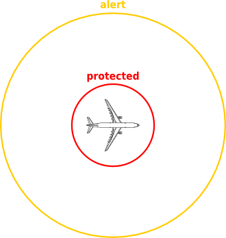
A conflict resolution manouever is considered when two planes have entered into each other’s alert zones. The system aims to ensure that neither plane ever enters the other’s protected zone.
In the model, the position and heading of Aircraft1 define, respectively, the origin and direction of the positive x-axis of a relative coordinate system, in which the position of Aircraft2 is specified. The heading of Aircraft2 is specified relative to the positive x-axis.
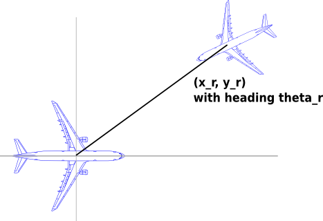
The initial condition in the model is that the aircraft are cruising outside each other’s protected zones, but inside each other’s alert zones.
The manouever modelled in this case is (taken directly from the paper):
Cruise
Cruise until aircraft are
alpha1miles apart.Left
Make a heading change of
delta_phiand fly until a lateral displacement of at leastdmiles is acheived for both aircraft.Straight
Make a heading change to the original heading and fly until the aircraft are
alpha2miles apart.Right
Make a heading change of
-delta_phiand fly until a lateral displacement of d miles is acheived for both aircraft.Cruise
Make a heading change to original heading and cruise.
Note that, in the model at least, the heading changes occur simultaneously and instantaneously.
(*
 * This example is taken from the paper:
 *   "Conflict Resolution in Air Traffic Management; A Study in Multiagent
 *    Hybrid Systems", Tomlin, Pappas, Sastry, 1998
 *)

(** constants, initial state **)

(* increase the derivatives for a faster animation *)
let tscale x = 20.0 *. x


let pi = 4.0 *. atan 1.0

let d = 10.0                (* distance to deviate for avoidance, in miles *)
let delta_phi = (pi /. 4.0) (* change in heading for avoidance, radians *)

let radius_protected = 5.0  (* radius of the protected zone, in miles *)
let radius_alert = 25.0     (* radius of the alert zone, in miles *)

let alpha1 = 16.0           (* distance at which avoidance is triggered *)
let alpha2 = 20.0           (* distance at which avoidance is terminated *)

(* velocity in miles/hour converted to miles/minute *)
let aircraft1_v = 540.0 /. 3600.0 (* velocity of aircraft1 *)
let aircraft2_v = 570.0 /. 3600.0 (* velocity of aircraft2 *)

(* initial position of aircraft2, relative to aircraft1 *)
let aircraft2_xi = 60.0
let aircraft2_yi = 28.0
let aircraft2_thetai = -. 3.0 *. pi /. 4.0

(** algorithm **)

let rotate (theta, x, y) = (x', y') where
  rec cos_theta = cos(theta)
  and sin_theta = sin(theta)
  and x' = (cos_theta *. x) +. (-. sin_theta *. y)
  and y' = (sin_theta *. x) +. (cos_theta *. y)

let rotate_x (theta, x, y) = (cos(theta) *. x) +. (-. sin(theta) *. y)
let rotate_y (theta, x, y) = (sin(theta) *. x) +. (cos(theta) *. y)

let sqr x = x *. x

let hybrid avoidance (x_i, y_i, theta_i, v_1, v_2) = (st, x, y, theta, show_t)
  where
  rec init theta = theta_i
  and der x = tscale (-. v_1 +. v_2 *. cos(theta))
              init x_i reset nxy(nx, _) -> nx
  and der y = tscale (v_2 *. sin(theta))
              init y_i reset nxy(_, ny) -> ny
  and der t = tscale t' init 0.0

  and automaton
      | Cruise ->
          do
            t' = 0.0
            and st = 0
            and show_t = 0.0
          until up(sqr(alpha1) -. sqr(last x) -. sqr(last y))
            then do emit nxy = rotate(-. delta_phi, last x, last y)
            in Left(d /. ((max v_1 v_2) *. sin(delta_phi)))
      | Left(tmax) ->
          do
            t' = 1.0
            and st = 1
            and show_t = t /. tmax
          until up(t -. tmax) then do
            emit nxy = rotate(delta_phi, last x, last y) in Straight(tmax)
      | Straight(tmax) ->
          do
            t' = 0.0
            and st = 2
            and show_t = t /. tmax
          until up(sqr(last x) +. sqr(last y) -. sqr(alpha2))
            then do emit nxy = rotate(delta_phi, last x, last y) in Right(tmax)
      | Right(tmax) ->
          do
            t' = -. 1.0
            and st = 3
            and show_t = t /. tmax
          until up(-. t)
            then do emit nxy = rotate(-. delta_phi, last x, last y) in Cruise

let hybrid noavoidance (x_i, y_i, theta_i, v_1, v_2) = (0, x, y, theta, t) where
  rec theta = theta_i
  and der x = tscale (-. v_1 +. v_2 *. cos(theta)) init x_i
  and der y = tscale (v_2 *. sin(theta)) init y_i
  and t = 0.0

(** Animation **)

open Airtrafficgui

let hybrid main () = () where
  rec p = period (0.1 | 0.1)

  and (click, (nxr, nyr), (ntheta_r, nd)) =
    present p -> sample ()
    init (false, (aircraft2_xi, aircraft2_yi), (aircraft2_thetai, 0.0))

  and automaton
	S1 ->
	  do
            (st, xr, yr, theta_r, t) =
               avoidance (nxr, nyr, ntheta_r, aircraft1_v, aircraft2_v)
          until p on click then S1

  and _ = present p -> showupdate (d, delta_phi, radius_alert,
                                   radius_protected, 0.0,
                                   st, xr, yr, theta_r,
                                   aircraft1_v *. 3600.0,
                                   aircraft2_v *. 3600.0, t)